Chapter 7Solution Structures of Native and Denatured Proteins Using RDCs
In the previous chapters, we introduced the principles of the Residual dipolar coupling (RDC), which can provide global orientational restrains on internuclear vectors. In this lecture, we introduce some RDC applications, that is, using RDCs to determine the solution structures of native [1, 2] and denatured [3] proteins.
Determining Native Protein Structure
We first introduce a quartic equation and two simple trigonometric equations that can compute, exactly and in constant time, the backbone dihedral angles for a residue from RDCs in two media on any single backbone vector type. Furthermore, based on these exact solutions we introduce a systematic search algorithm for determining protein backbone substructure consisting of both -helices and -sheets [1]. “Exact” solutions is a mathematical term, meaning that the polynomials can be solved in closed form (see chapters 15,16). It should not be confused with a guarantee of “biological exactness.”
Theoretical Background
Based on the equations of NH RDCs measured in two media, we can derive a quartic equation that allows us to compute the vector orientation. For instance, let be the NH bond vector in the POF of medium 1. With respect to , we have
where the coefficients , as well as and can be computed from the equations of NH RDCs (appendix A in [1]). As shown in figure 7.1, the number of real solutions of equation (7.1) is at most 8, or in other words, given NH RDCs measured in two media, we can obtain up to 8 possible vector orientations, one of which is the correct orientation.
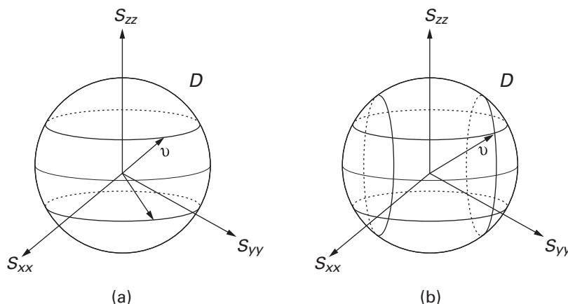
Figure 7.1 An example of extracting NH unit vector using RDCs in two media: (a) unit vector determined by one RDC; (b) unit vector determined by two RDCs. Consequently, 0, 2, 4, 6, or 8 solutions for the internuclear vector orientation can be obtained from two RDCs. Credit: Bruce Donald and Jeff Martin.
In order to compute the dihedral angles for a single residue, we can prove that if the directions of any two vectors and in consecutive peptide planes and are known, together with the orientation of peptide plane , then the intervening backbone angles can be computed from the following two trigonometric equations:
where , and are computed from the six bond angles between two consecutive residues, , and . The full expressions for all these four coefficients are computed from backbone kinematics (appendix B in [1]). Note that these two equations can be solved exactly for and , and therefore at most two possible solutions exist for each orientation of the pair of bond vectors.
Furthermore, if the first peptide plane is given, we can in principle compute all the possible angles of a fragment based on the following two observations: (1) A peptide plane with respect to a principal order frame (POF) for medium 1 can be determined by its vector and its NH vector; (2) a unique vector for the peptide plane can be computed from the vector of the peptide plane and . Therefore, we can consecutively compute all the possible discrete solutions for all the residues of the fragment by using a depth-first search (DFS) strategy. The optimal solution, under a scoring function, may be computed by DFS plus backtracking.
The Algorithm
The algorithm for determining a 3-dimensional backbone substructure containing -helices and -sheets employs the following inputs: (1) assigned backbone NH RDCs in two media,
- identified -helices and -sheets with known H-bonds between paired strands, and (3) very sparse NOE distance restraints. The algorithm is divided into three stages:
Computation of alignment tensors Using an ideal helix model built with the backbone, the Saupe matrices for both media can be computed from the model by SVD (chapters 4, 5). This is essentially a bootstrapping method to obtain initial estimates of the alignment tensors. The tensors are refined by refitting with SVD either during or after step 2 below. Then, an optimal first vector is computed using an -residue fragment built with the average dihedral angles from either an -helix or a -strand, and standard bond lengths and angles, using a grid search method over .
Refinement of secondary structure elements If the orientation of the first peptide plane of an -residue secondary structure element is given, the conformation can be specified uniquely by a sequence of backbone dihedral angles. We refine the fragment by optimizing both the directions of individual NH vectors and also the dihedral angles of the fragment using RDCs alone, while leaving the bond lengths and the six bond angles fixed. Furthermore, the plausible conformations are computed from a DFS-based refinement method, in which every computed pair is filtered through the favorable Ramachandran regions for the corresponding secondary structure type. Consequently, an optimal conformation is computed from the set of all the plausible conformation vectors using the scoring function defined in Wang and Donald [1].
Backbone structure determination We employ a few NOE-derived distances, including the distances between an amide proton and a nucleus or between two nuclei, to compute the relative position of the helix and the single sheet of ubiquitin.
Results
The work [1] has been successfully extended to compute a complete backbone structure [2], including turns and loops (connecting the secondary structure elements) using only NH and CH RDCs in a single medium (i.e., only two RDCs per residue) and two unambiguous NOEs. Here, CH means . Figure 7.2a shows the computed structure of ubiquitin backbone without loops, and figure 7.2b compares the computed structure of ubiquitin backbone with loops vs. a reference structure (see plate 2).
A discussion of the one-medium case (exact solutions from NH and CH RDCs in one medium) can be found in [4], where these algorithms were used prospectively to determine the NMR solution structure of the FF domain 2 of human transcription elongation factor CA150 (RNA polymerase II C-terminal domain interacting protein), PDB id: 2kiq [4].
Determination of Denatured or Disordered Proteins
In this section, we introduce a data-driven algorithm capable of computing a set of structures for denatured or disordered proteins directly from sparse experimental restraints, including the orientational restraints from RDCs, and distance restraints from paramagnetic relaxation enhancement (PRE) experiments.
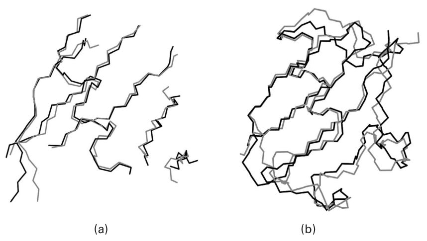
Figure 7.2 (plate 2) (a) Structure of ubiquitin backbone without loops. The ubiquitin backbone structure (blue) was computed using 37 NH and 39 CH RDCs, 12 hydrogen bonds, and four NOEs; (b) structure of ubiquitin backbone with loops. The ubiquitin backbone structure (blue) was computed by extending the algorithm to handle loop regions along the protein backbone. The structure was computed using 59 NH and 58 CH RDCs, 12 H-bonds, and two unambiguous NOEs. A reference structure (from crystallography) is shown (red).
A Probabilistic Interpretation of Restraints in the Denatured State
In contrast to the traditional algorithms for the structure determination of native proteins, Wang et al. [3] employ a set of tensors to interpret the RDCs measured in the denatured state. Each tensor in the set represents a cluster of similar denatured structures, and the set of RDCs corresponding to each tensor is sampled from the individual distributions associated with each measured RDC. That is, the experimentally measured RDC value in the denatured state is the expectation, and the different clusters of tensors represent different conformations that are oriented differently in the aligning medium. Similarly, the PRE-derived distance is also considered a random variable, where the measured value is an average over all the possible structures in the denatured state. Hence, the structure determination problem for denatured proteins can be formulated as the computation of a set of conformation vectors, given the distributions of all the RDCs and PREs.
The Algorithm
For a denatured protein, the algorithm in [3] computes a presumably heterogeneous ensemble of structures that are consistent with the experimental data within a large range. The input of the algorithm includes the protein sequence, at least two RDCs per residue in a single medium and PREs. For efficiency, a divide-and-conquer strategy is used in the algorithm to compute the ensemble, which consists of six steps (figure 7.3):
- Fragment division The entire protein sequence is divided into fragments and linkages , where a linker consists of the residues between two neighboring fragments.
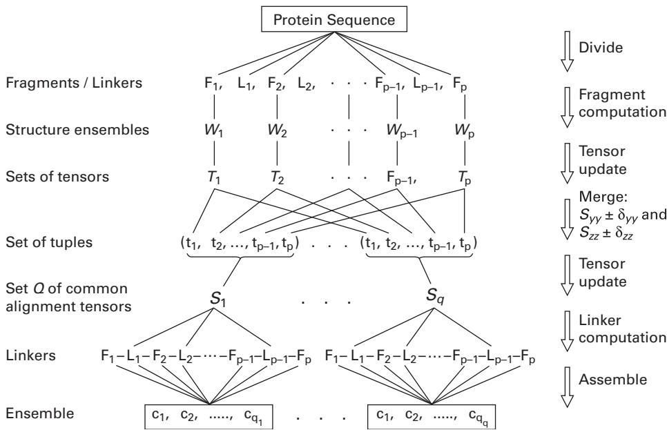
Figure 7.3 Divide-and-conquer strategy. The terms denote conformation vectors for the complete backbone structure.
- Fragment computation The algorithm computes an ensemble of structures for each fragment , independently.
- Tensor computation For each structure in ensemble , the corresponding tensor is computed by SVD and saved into a set . The SVD procedure is to minimize the RMSD between the experimental RDC data and the RDC back-computed from the structure using the tensor.
- Tensor merge All the tensors in the sets are merged into -tuples, , where is from the set . All the tensors in a -tuple have their and (two of three diagonal elements of the diagonalized Saupe matrix) values in the certain ranges of and , where and are thresholds.
- Tensor update For each merged -tuple, the algorithm computes their common tensor by SVD using the corresponding structures in and all the experimental RDCs for the fragments . Note that the SVD computation can output not only the diagonal elements , but also the orientation for each fragment in the common POF as well.
- Linker computation and assembly The algorithm computes each linker using every common tensor and assembles the corresponding fragments and linkers into complete backbone structures.
Applications to Biological Systems
The algorithm described in Wang and Donald [3] has been applied to compute the structure ensembles of two proteins, an acid-denatured ACBP and a urea-denatured eglin C, from experimental NMR data. For acid-denatured ACBP, an ensemble of 231 structures was computed at pH 2.3, and all the structures have no vdW repulsion larger than 0.1 Å except for a few vdW violations as large as 0.35 Å between the two nearest neighbors of a proline and the proline itself. Further analysis indicates that acid-denatured ACBP is neither random coil nor nativelike. The work [3] also drew a similar conclusion for the urea-denatured eglin C, for which an ensemble of 160 structures was computed in 8 M urea.
References
- [1] L. Wang and B. R. Donald. Exact solutions for internuclear vectors and backbone dihedral angles from NH residual dipolar couplings in two media, and their application in a systematic search algorithm for determining protein backbone structure. Journal of Biomolecular NMR, 29(3) (2004): 223–242.
- [2] L. Wang, R. Mettu, and B. R. Donald. A polynomial-time algorithm for de novo protein backbone structure determination from NMR data. Journal of Computational Biology, 13(7) (2006): 1276–1288.
- [3] L. Wang and B. R. Donald. A data-driven, systematic search algorithm for structure determination of denatured or disordered proteins. The Computational Systems Bioinformatics Conference (CSB), Stanford, CA (August 2006), pp. 67–78.
- [4] J. Zeng, J. Boyles, C. Tripathy, L. Wang, A. Yan, P. Zhou, and B.R. Donald. High-resolution protein structure determination starting with a global fold calculated from exact solutions to the RDC equations. Journal of Biomolecular NMR, 45(3) (2009): 265–81.