Chapter 11Computational Protein Design
This chapter introduces the automated protein design and experimental validation of a novel designed sequence, as described in Dahiyat and Mayo [1].
Introduction
Given a three-dimensional (3D) backbone structure, the protein design problem is to find an optimal sequence that satisfies the physical chemical potential functions and stereochemical constraints. Protein design is an “inverse folding problem,” and fundamental for understanding the protein function.
The term rotamer denotes discrete rotational conformations of protein side-chains. Typically these are represented by a finite discretization of the side-chain dihedral angles. Rotamers are based on observed side-chain conformations from a statistical analysis of high-resolution crystal structures in the PDB. A rotamer can encode a different conformation of the same amino acid side-chain, or a switch in amino acid type. Both are encoded uniformly using a rotamer library that contains the low-energy side-chain conformations across different amino acids.
The most basic protein design problem is often viewed as a search for the optimal rotamers to fit on a given protein backbone. Typically, the - bond remains invariant unless the residue is mutated to glycine or proline. The search returning the optimal rotamers yields both side-chain conformations and underlying design sequence. The sequence of the computed rotamers can be obtained by examining the amino acid type of each residue while disregarding its side-chain conformation. However, structural confirmation of a designed structure requires comparing the predicted side-chains (and backbone) versus the experimentally-determined structure by X-ray crystallography or NMR.
Overview of Methodology
The following is the methodology used in Dahiyat and Mayo [1]:
Given a backbone fold of a target structure, Dahiyat and Mayo [1] first developed an automated side-chain rotamer selection algorithm to (1) screen all possible amino acid sequences, and
- find the optimal sequence and side-chain orientations (rotamers). Then experimental validation by using NMR was performed to evaluate the computed optimal sequence/structures.
Algorithm Design
Input Backbone fold (Zif268), represented by structure coordinates. Here, “Zif” stands for “zinc finger.”
Output Optimal sequence (FSD-1). “FSD” stands for “full sequence design”; FSD-1 was the first full-length protein sequence to be designed by computational structure-based algorithms.
Overview
- The algorithm considers specific interactions between (a) side-chain and backbone and (b) side-chain and side-chain.
- The algorithm scores a sequence arrangement, based on a van der Waals potential function, solvation, hydrogen bonding, and secondary structure propensity [1].
- The algorithm considers a discrete set of rotamers, which are all allowed conformers of each side-chain.
- The algorithm applies a dead-end elimination (DEE) algorithm to prune rotamers that are inconsistent with the global minimum energy solution of the system.
Details The inputs of the algorithm are structure coordinates of the target motif’s backbone, such as N, Cα, C’, and O atoms, and Cα-Cβ vectors. The residue positions in the protein structure are partitioned into core, surface, and boundary classes. The set of possible amino acids at the core positions is {Ala, Val, leu, Ile, Phe, Tyr, Trp}. The set of amino acids considered at the surface positions is {Ala, Ser, Thr, His, Asp, Asn, Glu, Gln, Lys, Arg}. The combined set of both core and surface amino acids are considered for the boundary positions.
Note The total number of possible amino acid sequences is equal to the product of possible amino acids at each residue position. For instance, suppose that there are 7 possible amino acids at one core position, and 16 possible amino acids at each of 7 boundary positions, and 10 possible amino acids at each of 18 surface positions. The search space consists of possible amino acid sequences.
The algorithm is divided into two phases:
Phase 1 (Pruning) The algorithm applies DEE to find and eliminate rotamers that are dead-ending with respect to the global minimum energy conformation (GMEC). A rotamer at residue position will be eliminated (i.e., proven to be dead-ending) if there is another rotamer at the same position such that replacing by will always reduce the energy. However, naïvely checking this will still take exponential time. Therefore, the following pruning was applied. Below, denotes rotamer at sequence position . Similarly, and denote, respectively, rotamer at position , and rotamer at position .
DEE Condition If there exists a rotamer satisfying
then will be eliminated, where and represent self-energies, that is, energies between the atoms of a single rotamer (e.g., ). By convention, and for convenience, we include in the self-energy term the rotamer-template energies also. In this context, “template” means the geometric structure of the protein backbone atoms. and represent residue pairwise, rotamer-rotamer energies for rotamers , and . The condition in equation (11.1) ensures that replacing by will always reduce the energy, regardless of what the rotamers at other residue positions are. The intuition behind equation (11.1) is given in section 11.4.
Note that we have “overloaded” the operator to represent both self-energies (e.g., ) and residue-pairwise energies (e.g., ). Many protein design algorithms (including most of those in this book) explicitly require that the energy function be residue-pairwise additive. The DEE algorithms directly exploit this assumption. In general, DEE algorithms could, in principle, be extended to work with residue- -wise additive energy functions instead, for a small constant . However, parameterizing such energy functions requires care, and can be difficult. In general, “N-body” energy functions (where N is the total number of atoms) such as the Generalized Born/Poisson-Boltzmann solvation models are not amenable to DEE. However, there are approximate pairwise solvation models, and these are discussed in chapter 12.
Different scoring functions are defined for core, surface, and boundary residues separately. The scoring function for core residues uses “a van der Waals potential to account for steric constraints and an atomic solvation potential favoring the burial and penalizing the exposure of nonpolar surface area” [1]. The surface residues apply a hydrogen-bond potential and secondary structure propensities, and a van der Waals potential. The residues at the boundary positions use a combination of both core and surface scoring functions. The details of these scoring functions, and how they are combined, are sketched in [1], but are discussed at length in a U.S. Patent [7]. Further discussion of empirical molecular mechanics energy and scoring functions is given in chapter 12.
Phase 2 (Enumeration) For any residue position , let be the set of remaining rotamers that are not eliminated in Phase 1. The algorithm then enumerates all the combinations of remaining rotamers—that is, —to find the combination that has the global minimal energy. Enhancements to DEE (e.g., [3, 2]) also prune pairs of rotamers that are inconsistent with the GMEC, returning only subsets of the pairwise cross products. Rotamer pairs in but outside cannot participate in the GMEC.
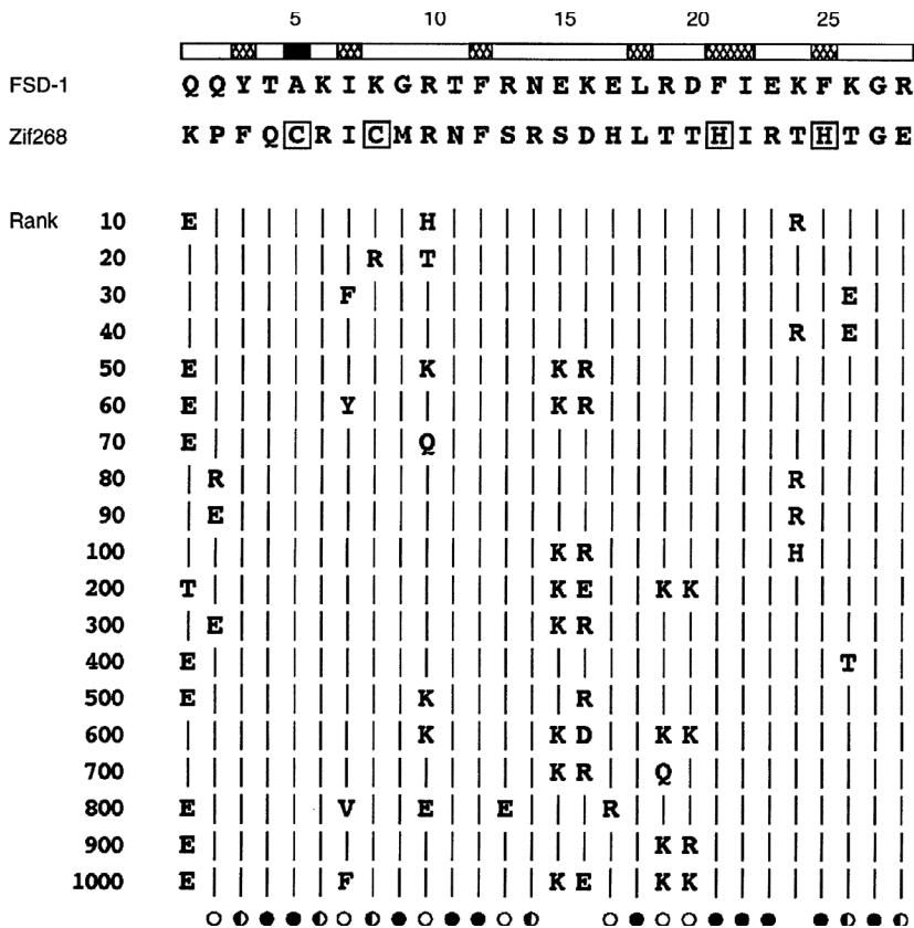
Figure 11.1 Comparison of computed sequence FSD-1 and the target sequence Zif268 [1]. Sequence of FSD-1 aligned with the second zinc finger of Zif268. The bar at the top of the figure shows the residue position and the open bars indicate the 20 surface positions. The alignment matches positions of FSD-1 to the corresponding backbone template positions of Zif268. Of the six identical positions (21 percent) between FSD-1 and Zif268, four are buried (lle7, Phe12, Leu18, and lle22). The zinc-binding residues of Zif268 are boxed. Representative nonoptimal sequence solutions determined by means of a Monte Carlo simulated annealing protocol are shown with their rank. Vertical lines indicate identity with FSD-1. The symbols at the bottom of the figure show the degree sequence conservation for each residue position computed across the top 1,000 sequences: filled circles indicate more than 99 percent conservation, half-filled circles indicate conservation between 90 and 99 percent, open circles indicate conservation between 50 and 90 percent, and the absence of a symbol indicates highest occurrence at each position is identical to the sequence of FSD-1. Single-letter abbreviations for amino acid residues as follows: A, Ala; C, Cys; D, Asp; E, Glu; F, Phe; G, Gly; H, His; I, lle; K, Lys; L, Leu; M, Met; N, Asn; P, Pro; Q, Gln; R, Arg; S, Ser; T, Thr; V, Val; W, Trp; and Y, Tyr [1]. Reprinted with permission from AAAS.
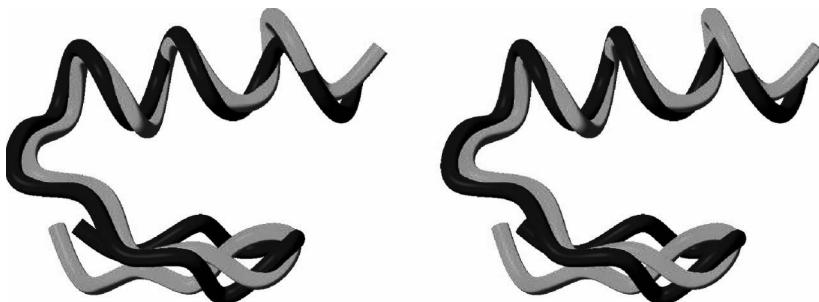
Figure 11.2 (plate 9) Backbone structure comparison of computed sequence FSD-1 and the target sequence Zif268 [1]. Comparison of the FSD-1 structure (blue) and the design target (red). Stereoview of the best-fit superposition of the restrained energy minimized average NMR structure of FSD-1 and the backbone of Zif268. Residues 3 to 26 are shown. [1]. Reprinted with permission from AAAS.
Phase 1 is provably correct, in that no rotamer will be pruned if it is part of the GMEC. Phase 1 is also polynomial-time. Phase 2 can be made provable using the search algorithm (chapter 12 and [4]). That is, after DEE will guarantee to compute the GMEC. Phase 2 is worst-case exponential-time.
Results Figure 11.1 shows the comparison of optimal computed sequence FSD-1 and the target sequence Zif268. Figure 11.2 (plate 9) compares the experimentally determined structure of the optimal computed sequence FSD-1 versus the structure of the target backbone sequence Zif268.
Intuition: Dead-End Elimination
Here is the intuition behind equation (11.1), the Dead-End Elimination (DEE) condition. We repeat it here for clarity:
Recall that lower energy is better; we are searching for the GMEC. The DEE condition (equation 11.1) tells us that we can prune a candidate rotamer if certain conditions hold. Those conditions include: the existence of a competitor rotamer (i.e., a competitor rotamer , also at position ) that is better than . But how can we prove that is better than ? For this calculation, it will be helpful to use the perspective of a witness rotamer . In this biophysical modeling problem, the only “perspective” a witness can have on the discrete choice versus is its energetic interaction with the candidate versus the competitor. One of these energies will be more favorable, which implies we may construct a penalty for the choice of rotamer versus at position .
First, the DEE condition contains a local side-chain-backbone penalty encoding the cost of choosing versus . This is . It is independent of .
The DEE condition also includes a pairwise side-chain-side-chain penalty for the cost of choosing versus , from the perspective of . Now, if we knew what rotamer was at position , then this penalty would simply be . Since we don’t, all possible rotamers at position must be considered. The pairwise penalty is built by computing at position a lower bound on the versus penalty, namely, . The minimization occurs over all possible rotamers at position . Then a sum is computed of all such lower bounds over all residue positions: . If the entire quantity on the left-hand side in equation (11.1) is positive, then rotamer can be pruned, since we have proven it cannot participate in the GMEC.
Finally, the DEE criterion can be efficiently computed, in polynomial time, by enumerating triples of the form . We prove this below.
Complexity Analysis
Let denote the number of residues, and denote the (maximum) number of possible rotamers for each residue.
We first analyze the time complexity of DEE pruning in phase 1. For each rotamer at a specific residue position , it takes time to search all possible amino acids in all other positions to find . Comparisons with other rotamers at the same position take time. Since we need to consider all possible rotamers at every position , the total DEE pruning takes time. So DEE is polynomial time!
Although the pruning step will eliminate many states (that is, many configurations of rotamers) in the search space, it cannot guarantee that the number of the remaining states is small enough for the enumeration to be efficient. Even if there are only two rotamers remaining for each position, the worst-case time to find the state that minimizes the energy is still exponentially large.
Note In fact, the optimization problem of finding the GMEC in protein design has been proven NP-hard [5], and even NP-hard to approximate [6].
Experimental Validation: Interplay of Computational Protein Design and NMR
The solution structure for the computed sequence FSD-1 was obtained by using 2D NMR spectroscopy. Sample NMR data, including a NOESY spectrum, are shown in figure 11.3. X-PLOR plus the standard protocols for hybrid distance geometry-simulated annealing were used to calculate the structure. Table 11.1 and Figure 11.4 (plate 10) show an ensemble of 41 structures that are consistent with good geometry and distance constraints within a small tolerance. The structure of FSD-1 was close to the target structure (Zif268), validating the structure-based protein design algorithm using DEE.
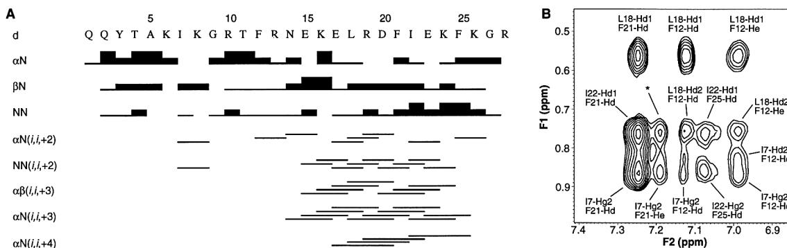
Figure 11.3 NMR data for FSD-1: (a) FSD-1, sequential and short-range NOE connectivities. The “d” denotes a contact between the indicated protons. All adjacent residues are connected by -HN, -HN, or -HN NOE crosspeaks. The helix (residues 15 to 26) is well-defined by short-range connections, as is the hairpin turn at residues 7 and 8; (b) 2D NOESY spectrum for the optimal computed sequence FSD-1. Several long-range NOEs from and to the helix help define the fold of the protein. The starred peak has an ambiguous assignment, or [1]. Reprinted with permission from AAAS.
Table 11.1 NMR structure determination of FSD-1: distance restraints, structural statistics, and atomic root-mean-square (rms) derivations
| Distance restraints | ||
|---|---|---|
| Intraresidue | 97 | |
| Sequential | 83 | |
| Short range ($ i - j = 2$ to 5 residues) | 59 | |
| Long range ($ i - j > 5$ residues) | 35 | |
| Hydrogen bond | 10 | |
| Total | 284 | |
| Structural statistics | ||
| rms deviations | ||
| Distance restraints () | 0.038 | |
| Idealized geometry | ||
| Bonds () | 0.0037 | |
| Angles (degrees) | 0.65 | |
| Impropers (degrees) | 0.51 | |
| Atomic rms deviations ()* | ||
| versus | versus | |
| Backbone | ||
| Backbone + nonpolar side-chains† | ||
| Heavy atoms |
*Atomic rms deviations are for residues 3 to 26, inclusive. Residues 1, 2, 27, and 28 were disordered [ , , angular order parameters (34) ] and had only sequential NOEs. †Nonpolar side-chains are from residues , , , , , , , and , which constitute the core of the protein. (SA) are the 41 simulated annealing structures, SA is the average structure before energy minimization, are the restrained energy minimized average structure, and SD is the standard deviation.
Source: [1]. Reprinted with permission from AAAS.
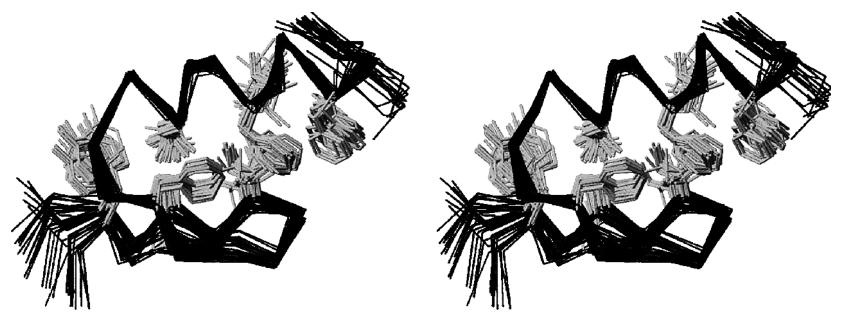
Figure 11.4 (plate 10) Empirically determined NMR structure ensemble of FSD-1, including side-chains. Stereoview showing the best-fit superposition of the 41 converged simulated annealing structures from XPLOR. The backbone trace is shown in blue and the side-chain heavy atoms of the hydrophobic residues ( , , , , , , , and ) are shown in magenta. The amino terminus is at the lower left of the figure and the carboxyl terminus is at the upper right of the figure. The structure consists of two antiparallel strands from positions 3 to 6 (back strand) and 9 to 12 (front strand), with a hairpin turn at residues 7 and 8, followed by a helix from positions 15 to 26. The termini, residues 1, 2, 27, and 28 have very few NOE restraints and are disordered [1]. Reprinted with permission from AAAS.
The structure determination in [1] also represents a simple didactic example of the classic method of NMR protein structure determination in the solution state, based primarily on NOEs. Hence, this experimental study illustrates the biophysical concepts introduced in the preceding chapters on NMR. Although FSD-1 is a small protein, the basic concepts such as sequential and short-range NOEs, NOESY crosspeaks, NOESY assignment, structural ensembles, and the simulated annealing structure determination protocols, are illustrated in this study. For example, note the ambiguous NOESY crosspeak assignment (*) in figure 11.3b. The NOE patterns exploited by the JIGSAW algorithm (chapter 8) are clearly seen in figure 11.3a.
This example of NMR structure determination in the solution state is a special and restricted case, in which FSD-1 could be synthesized through solid-phase -fluoren-9-ylmethoxycarbonyl (Fmoc) chemistry. A modern study of a larger protein would typically employ stable isotopic labeling by recombinant protein expression in a bacterial host (such as E. coli) followed by protein purification by fast protein liquid chromatography (FPLC), and additional NMR experiments (e.g., triple-resonance, IPAP) for assignments and to measure structural restraints such as RDCs in weakly aligned conditions (chapters 15–18). Nevertheless, these results represent a successful end-to-end study using the techniques we have been discussing, including algorithms for protein design and NMR structural biology.
References
- [1] B. I. Dahiyat and S. L. Mayo. De novo protein design: Fully automated sequence selection Science 278;5335 (1997 October 3):82.
- [2] J. Desmet J, De Maeyer M, and Lasters I. Theoretical and algorithmical optimization of the dead-end elimination theorem. Pacific Symposium on Biocomputing (1997):122–133. PubMed PMID: 9390285.
- [3] I. Lasters, M. De Maeyer, and J. Desmet. Enhanced dead-end elimination in the search for the global minimum energy conformation of a collection of protein side-chains. Protein Engineering (1995) Aug;8;8:815–822.
- [4] A. Leach and A. Lemon. Exploring the conformational space of protein side-chains using dead-end elimination and the algorithm. Proteins, 33:227–239, 1998.
- [5] Niles Pierce and Erik Winfree. Protein design is NP-hard. Protein Engineering, 15 (2002):779–782.
- [6] Bernard Chazelle, Carl Kingsford, and Mona Singh. A semidefinite programming approach to side-chain positioning with new rounding strategies. INFORMS Journal on Computing, 16;4 (2004):380–392.
- [7] S.L. Mayo et al. “Apparatus and Method for Automated Protein Design.” U.S. Patent 6,269,312 (2001).