Chapter 14Nuclear Vector Replacement
This lecture presents the nuclear vector replacement (NVR) algorithm, and its applications in automated NMR resonance assignments [1, 2] and three-dimensional (3D) structural homology detection [3, 4]. The expectation-maximization approach is introduced, which complements bipartite matching as a useful framework for many structural problems.
NVR stands for “Nuclear Vector Replacement.” It is named by analogy to “molecular replacement” in X-ray crystallography (chapters 47 and 48).
Experimental Input
NVR is an algorithm for computing resonance assignments given a putative 3D structural model of the target protein. This model is typically a PDB format structure. The following data are processed in the NVR algorithm: unassigned chemical shifts in HSQC spectra, RDCs in two media, amide exchange data, and unassigned peaks in 3D -NOESY spectra. The amide exchange information provides probabilistic classifications for the peaks in the HSQC corresponding to non-hydrogen-bonded, solvent-accessible backbone amide protons. All the RDC, H-D exchange and -NOESY data serve as the geometric constraints on assignment. Table 14.1 shows the information content and roles of the input data.
Nuclear Vector Replacement
The NVR algorithm consists of three phases: tensor estimation, resonance assignment, and structure refinement, as shown in figure 14.1. In the first phase, NVR estimates the alignment tensors in both media. In the second phase, NVR applies the estimated tensors, and uses an iterative computational process, such as a Bayesian or expectation/maximization framework, to search the optimal resonance assignments. After resonance assignments, the assigned RDCs are used to refine the structure of the model by using the algorithm in Wang and Donald [6]. In the following subsections, we will present more details on the tensor estimation and resonance assignment phases.
Table 14.1 Information contents and roles of the input data [1]
| Experiment/Data | Information Content | Role |
|---|---|---|
| HSQC | chemical shifts | Backbone resonances, cross-referencing NOESY |
| RDC (in 2 media) | Restraints on amide bond vector orientation | Tensor determination, resonance assignment, |
| H-D exchange HSQC | Identifies solvent exposed amide protons | Tensor determination |
| HSQC-NOESY | Distance restraints between spin systems | Tensor determination, resonance assignment |
|
TOCSY Backbone structure Chemical shift predictions |
Side-chain chemical shifts Tertiary structure Restraints on assignment |
Tensor determination, resonance assignment Tensor determination, resonance assignment Tensor determination, resonance assignment |
Reprinted from [1]. Copyright 2004 IEEE.
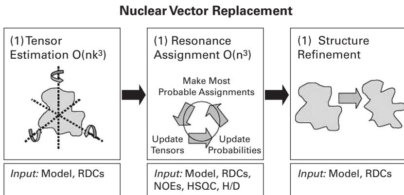
Figure 14.1 Nuclear vector replacement [2].
Tensor Estimation
An alignment tensor is a symmetric and traceless matrix with five degrees of freedom, for example, three Euler angles , and , and the axial and rhombic components of an ellipsoid scaling the dipolar couplings. The alignment tensor can be diagonalized as follows:
where is a rotation matrix that defines the principle order frame, and is a diagonal and traceless matrix containing the eigenvalues of and encoding and .
denotes the special orthogonal group of real invertible matrices. It is the intersection of the orthogonal group of orthogonal matrices, and the special linear group of matrices with determinant . is isomorphic to the group of three-dimensional rotations.
The diagonal elements of can be obtained based on the powder pattern method. Given , a rotation matrix , corresponding to an alignment tensor , is found such that the Kullback-Leibler distance is minimized between the distribution of unassigned experimental RDCs and the distribution of the back-computed RDCs.
Time Complexity The eigenvalues of are computed in time, where is the number of experimental RDCs and is the resolution of the search-grid over . The rotation matrix is calculated in time. Given and , constructing takes only time. Thus, the total running time for tensor estimation is . The Euler angle representation of three-dimensional rotations is familiar to many students; however, it suffers from singularities. A preferred representation of rotations is unit quaternions. Geometrically, quaternions may be represented by the three-dimensional sphere , which is a double cover of . That is, if is a quaternion, then we have a smooth map such that is the rotation by and . The quaternions, like the Euler angles, form a three-dimensional space () and therefore can be searched using three parameters (similar to ) to construct a grid over . Only half of must be searched, since .
Resonance Assignment
Based on the estimated tensors and in two alignment media, the back-computed RDCs are obtained according to the following equation:
where is the dipolar interaction constant, and is the internuclear vector orientation.
Let be the set of HSQC peaks, be the set of residues, be the set of experimental RDCs in the medium , and be the back-computed RDCs in the medium , based on . Let be the assignment probability matrix for the medium such that
where , , , , and denotes the normal distribution function with the observed variable , the mean , and the standard deviation . Each entry in will be set to zero if the assignment violates some geometric constraint, such as the from spectra, or amide exchange. The provide distance constraints between peaks that can be correlated to the residues in the model, while the H-D exchange information identifies fast-exchanging amide protons that are likely to be solvent-exposed and non-hydrogen-bonded, and can be correlated to the structure model.
Equation (14.2) is used to compute the assignment probability at each iteration. The most likely assignment in each medium is considered. Let be the most likely assignments of peak in media 1 and 2. The assignment is added into the master list of assignments if both following conditions are satisfied:
and
It is possible that the second condition is not satisfied. In this case, a maximum bipartite matching is chosen.
Suppose that peak has been assigned to , then and are removed from the consideration of next iterations. At the end of each iteration, the alignment tensors and are refined based on the master list of assignments and model. At the same time, the assignment probabilities are renormalized and updated.
Time Complexity It takes time to construct the probability matrices. Updating the alignment tensors and takes time. Since at least one residue is assigned at each iteration, there are at most iterations. Thus, all assignments are guaranteed to be finished in time. The time complexity has been improved to be in Langmead and Donald [5], where is the maximum edge-weight in an integer-weighted bipartite graph.
An Expectation/Maximization NVR Algorithm
Langmead and Donald [1] applied an expectation/maximization NVR algorithm for automated NMR resonance assignments. In the expectation/maximization framework, the observed variables include chemical shifts, , amide exchange rates. The hidden variables include the correct resonance assignments and the correct alignment tensors. Let be the set of observed variables, and be the set of hidden variables. Let denote the set of all assignments obtained so far. Initially, is set to be empty, and then grows as the algorithm finds more assignments. The Expectation (E) step of the EM algorithm computes the following expectation:
where denotes the set of new assignments that is disjoint with the previous set . The Maximization (M) step computes the new assignment that has the maximum likelihood:
At the same time, the algorithm updates the master list of assignment, that is, . Also, the alignment tensors are recomputed at the end of each iteration, based on updated assignments in . The algorithm terminates when all peaks have been assigned.
3D Structural Homology Detection via NVR
Given unassigned RDCs of a target protein and a set of known models (protein structures in PDB format) in a database, we measure the 3D structural homology between the target protein and each known model by computing the likelihood of the assignment from the experimental RDCs to the model. We run the NVR algorithm for each model in the database, and then rank them by the likelihoods of the assignments.
Time Complexity Suppose that there are in total models in the database. Since the NVR algorithm runs in time, processing all proteins takes . Finally, sorting all models according to their likelihoods of assignments takes time. Thus, the total required time is .
Matching Modulo a Group, and Clustering Modulo a Group
NVR for automated NMR resonance assignments can be viewed as a matching problem on a quotient space of (bond-vector) orientations, induced by a quadratic form on the 2-sphere . is given by the familiar RDC tensor equation (eq. 14.3):
from above. Using the alignment tensor , is parameterized by the Lie group . is traceless and symmetric. When the eigenvalues of can be experimentally estimated (as is often the case), the degrees of freedom reduce to . Hence, 3D structural homology detection from unassigned NMR data (enabling rapid fold determination) can be performed by combinatorial optimization, searching over to minimize a functional that compares distributions generated by ’s image of the bond vectors from putative database protein models (chapter 13). These algorithms are developed further in chapters 15–18.
Using the techniques in chapters 4, 13, and 15–18, the RDC equations can be combined with protein kinematics to reduce the problem of protein structure determination from RDCs, to a search over the (discrete and finite number of) roots of low-degree univariate polynomial equations. These techniques have been developed for NH RDCs in two media, and for NH and CH (i.e., -H ) RDCs in one medium. They can be extended to use alternative RDCs (on different bond vectors), additional RDCs, or additional aligning media.
In some cases, such as NH RDCs in two media, or NH and CH RDCs in one medium, solving the resulting polynomial equations (generically) results in multiple (albeit finite and discrete) roots. Hence, the structure determination algorithm must typically perform a discrete and combinatorial search for the correct root, i.e., the true solution.
In 3D structural homology detection, there are two ambiguities in matching: which bond vector, and which root. The following toy example illustrates the concept. We consider the case of NH
RDCs in two media. Suppose we have NH bond vectors in a putative structural model from only two residues, Arg25 and Phe53. Call these and , and without loss of generality consider them to be unit vectors lying on . Now, suppose from the NMR data there are two unassigned residues A and B, from which we compute roots and to the RDC equations. These roots define possible NH bond vectors for the two unassigned residues A and B. Thus, we will think of the NH bond vector of residue A as lying in the set . The NH bond vector of residue B lies in the set . Note that and each have four points (in this example) and therefore are discrete and finite subsets of . A legal matching has the form or , for . But all matches of the form and are illegal since in the first case and are roots of the same polynomial, and hence correspond to two possible but mutually exclusive choices for same bond vector based on the data. Similarly, and are both roots of a (different) polynomial, and correspond to mutually exclusive choices for a single bond vector in the data. If and are viewed as sets, then the legal matchings have a simple “XOR” (exclusive OR) structure. However, and have a group structure, since each is constructed from the roots of a polynomial. The group-theoretic viewpoint gives the problem a fascinating mathematical structure, that can likely be exploited by advanced algorithms. We call this problem matching modulo a group. It is worth explaining the terminology. If is the group of , then the intuition is, to say “ is the same as modulo ” signalizes that “ and are the same except for differences accounted for or explained by .” The word modulo is mathematical shorthand to denote equivalence in the orbit space . is the quotient of the group action on the manifold .
To summarize, in NVR, bond vector orientations from a putative structural model can be matched against the multiple roots of the RDC equations. Only one root-match per model bond vector can be correct. This problem may be viewed as matching modulo a group, where the group encodes the multiplicity of the roots, and is related to the Galois group of the RDC-kinematic polynomials derived by Wang and Donald (chapters 16, 17). While the problems of matching and clustering have received a great deal of attention in computer science, machine vision, and computational biology, the problems of matching modulo a group and clustering modulo a group are relatively new, and are of considerable biological and computational importance. Clustering modulo a group will be discussed later, in chapter 47.
References
- [1] C. J. Langmead and B. R. Donald. An expectation/maximization nuclear vector replacement algorithm for automated NMR resonance assignments. Journal of Biomolecular NMR 29;2(2004):111–138.
- [2] C. J. Langmead, A. K. Yan, R. H. Lilien, L. Wang, and B. R. Donald. A polynomial-time nuclear vector replacement algorithm for automated NMR resonance assignments. RECOMB (2003): 176–187. Journal Computational Biology 11;2–3(2004):277–298.
- [3] C. J. Langmead and B. R. Donald. 3D structural homology detection via unassigned residual dipolar couplings. Proceedings of IEEE Computational Systems Bioinformatics Conference (CSB), Stanford University, Palo Alto (August 10, 2003), pp. 209–217.
- [4] C. J. Langmead and B. R. Donald. High-throughput 3D structural homology detection via NMR resonance assignment. Proceedings of IEEE Computational Systems Bioinformatics Conference (CSB), Stanford, (August, 2004), pp. 278–289.
- [5] C. J. Langmead and B. R. Donald. An improved nuclear vector replacement algorithm for nuclear magnetic resonance assignment. Tech. Rep. TR2004-494, Dartmouth Department of Computer Science, 2004.
- [6] L. Wang and B. R. Donald. Exact solutions for internuclear vectors and backbone dihedral angles from NH residual dipolar couplings in two media, and their application in a systematic search algorithm for determining protein backbone structure. Journal of Biomolecular NMR, 29;3(2004):223–242.