Chapter 36SemiDefinite Programming and Distance Geometry with Orientation Constraints
This chapter introduces Semidefinite programming and its applications in two areas: the side-chain positioning problem and the sensor network localization problem. We present the problem of distance geometry with orientation constraints: we first introduce the graph embedding problem with angle information, and then revisit the problem of protein backbone determination using the global orientational constraints from RDC data.
SemiDefinite Programming and Two Applications
Overview of SemiDefinite Programming
Semidefinite programming (SDP) has been one of the most exciting developments in mathematical programming since the 1990s [4]. Semidefinite programming is a special case of convex programming, in which we must optimize a linear function of symmetric matrices subject to linear equality constraints, and where the matrix must be positive semidefinite.1 For any additive error , semidefinite programs can be solved in polynomial time, in terms of both the size of input and , using the ellipsoid algorithm or interior-point method.
Application in the Side-Chain Positioning Problem
In the side-chain positioning problem (See chapters 11–12), we are given a backbone of length , and a set of side-chains , also called rotamers, for each residue position , and our objective is to find a sequence of side-chains that minimizes the following energy function:
where denotes the self-energy of the backbone, denotes the energy resulting from the interaction between the backbone and the rotamer at position , and denotes the energy resulting from the interaction between chosen rotamers and .
1 Suppose that is an matrix. Then is a positive semidefinite (PSD) matrix if for any .
The side-chain positioning problem can also be formulated in graph-theoretic terms. Let denote a -partite graph with node set , where represents the set of rotamers at position . Each node is associated with a weight . Each edge between nodes (corresponding to ) and (corresponding to ) () is assigned a weight . Now, the side-chain positioning problem is converted into the problem of finding a node per to minimize the weight sum of the induced subgraph.
The side-chain positioning problem has been proven to be NP-hard [5] and even hard to approximate [3]. It can be directly formulated into the following integer quadratic programming problem:
We next show how to relax this integer quadratic programming problem to a semidefinite programming formulation [3]. First, we add a new singleton vertex set, , into graph . The formulation in (36.1) can be converted into the following, equivalent program:
We relax the requirement to for all and , and then obtain the following semidefinite programming formulation:
We can obtain a solution of the preceding SDP system within any desired level of accuracy in polynomial time by using the ellipsoid algorithm or interior-point method. After that, we use a randomized rounding scheme to round each vector to 0 or 1. The basic idea is to sample each position from a specified probability distribution in which long vectors have a higher probability of being selected. For more details of the rounding scheme, see section 3 in Biswas et al. [2].
Application in the Sensor Network Localization Problem
It is interesting that SDP can also be used to solve the other problems, such as those in sensor networks. We give one example now.
In a sensor network in , we are given sensors and anchors. An anchor is a node whose position , , in is known. We also know , a set of Euclidean distances between two sensors and , and , a set of Euclidean distances between a sensor and an anchor . The sensor network localization problem is to find all , , that satisfy all the distance constraints
Let . Then the sensor network localization problem can be formulated into the following matrix form:
This form can be relaxed to a semidefinite program by changing constraint to . Here, the symbol means positive, semidefinite:
The -solution of this SDP system—that is, the solution within error distance from the optimal one—can be computed in time using the interior-point algorithm, where .
Distance Geometry with Orientation Constraints
We now discuss the graph embedding problem with local angle information, and then compare with the protein structure determination problem based on global RDC orientational constraints.
Graph Embedding with Angle Information
In space, the distance between two points and in -dimensional space is measured according to the norm, that is,
In a graph embedding problem, we are given a graph , and lengths for all edges . Our objective is to embed into a space by a map such that the following graph distortion is minimized:
Badoiu et al. [1] considered the embedding problem assuming multiplicative errors on edges and additive errors on angles. The naïve setup of the problem is nonconvex and difficult to solve. The following shows how to relax the problem to a convex problem at the cost of some error [1].
Consider a distance geometry problem with orientational restraints, where the angle of an edge with the -axis is given up to angular error . As shown in figure 36.1, the distance and angle information for the edge specifies a nonconvex feasible region for , given a fixed point . We can add an edge and relax the feasible region to be convex. Next, a linear program can be used to solve the problem in polynomial time. The maximum expansion error is, at most, after computing the maximum distance in the cutoff region.
Exercise 36.1 Compare the approximation algorithm above to the lower bounds in chapter 32 and [6], which prove there is an obstruction to obtaining an approximation for graph embedding without orientational constraints. How does the addition of this orientation information enable a provably good, polynomial-time approximation algorithm? In protein structure determination, how could such information be measured experimentally?
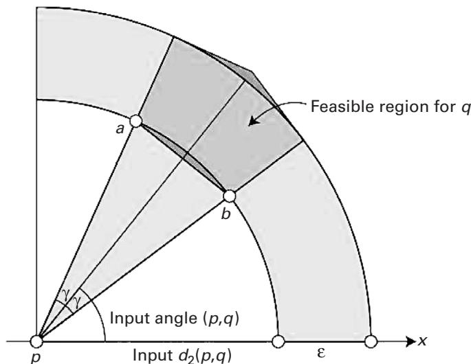
Figure 36.1 The relaxation in the embedding problem. Feasible region of a point with respect to given the distance within a multiplicative error and given the angle to the axis within an additive angular error [1].
Protein Structure Determination from RDCs
We close with an open problem. Let us review RDC-based protein structure determination (chapters 15–18). Given a bond vector , its corresponding RDC can be measured by
where is a physical constant, and is the alignment tensor.
Let be the coordinates of bond vector . We have
where , , and are the three diagonal elements of in the principal order frame.
Suppose we are given RDCs for a bond vector in two independent media, then we have the following relations:
where the third equation stands for the transformation relationship (a rigid rotation) between the two alignment tensors. This system is solvable, and by symmetry, there are up to 8 possible solutions (see chapters 15–18).
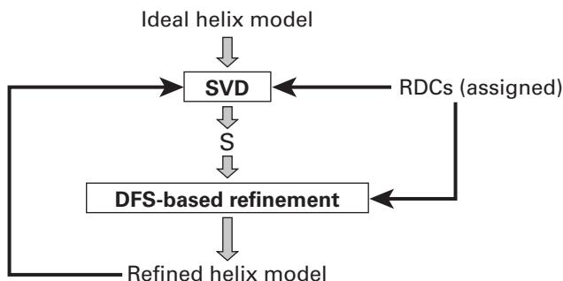
Figure 36.2 The computation of alignment tensors.
Suppose we are given N-H RDCs in two media for a peptide chain. We can compute all possible N-H bond vectors according to the preceding equations. If we can fix the position of the first peptide plane, there are two possible angles for each pair of bond vectors in two adjacent peptide planes, based on trigonometry and inverse kinematics computation. Thus, we have a discrete and finite set of all possible conformations for this peptide chain. However, two issues still remain to be addressed: First, how do we fix the first peptide plane, and second how do we compute the alignment tensors and . In [7], an ideal helix model is initially used to represent a helix in the protein structure, as shown in figure 36.2. Then an initial alignment tensor is calculated using SVD to fit , that is, minimize . Based on the computed alignment tensor, a DFS-based method is used to search for the structure, based on which we can recompute the alignment tensor. The orientation of the first peptide plane can be obtained based on the computed alignment tensor and two known bond vectors, N-C and N-H in the plane.
A divide-and-conquer strategy is used to determine the overall protein structure. We first divide the whole protein into several fragments (according to secondary structure elements). The conformation of each fragment can be computed based on the preceding protocol. Finally, we assemble all fragments by pure translations based on sparse NOE distance constraints.
Time Complexity Let denote the number of residue in the protein. The dividing step takes time. The structure determination of each fragment takes , where is the maximum length of fragments. The assembling step runs in time. Since [8], the total running time is . This algorithm is therefore optimal in terms of the geometric and combinatorial complexity . See chapters 15 through 18 and Wang et al. [8].
Open Problem RDCs are a geometric measurement similar to the angular restraints with error in figure 36.1 and section 36.2.1. Use SDP and the concept of distance geometry with angle restraints to model RDC-based structure determination. The angular restraints come from RDCs, and the distance restraints from NOEs. What is the best algorithm you can derive, in terms of complexity? Implement and test your algorithm, using both synthetic and real NMR data.
References
- [1] M. Badoiu, and E. D. Demaine, M. T. Hajiaghayi, and P. Indyk. Low-dimensional embedding with extra information. Proceedings of the Twentieth Annual Symposium on Computational Geometry, 2004.
- [2] P. Biswas and T. Lian and T. Wang, and Y. Ye. Semidefinite Programming based algorithms for sensor network localization. ACM Transactions on Sensor Networks (TOSN), (2006).
- [3] Bernard Chazelle, Carl Kingsford, and Mona Singh. A semidefinite programming approach to side-chain positioning with new rounding strategies. INFORMS Journal on Computing 16;4(2004): 380–392.
- [4] R.M. Freund, Introduction to Semidefinite Programming. Sloan School, MIT, DSPACE online publication (1999) accessed: 2009, url: http://dspace.mit.edu/bitstream/handle/1721.1/35259/15-094Spring-2002/NR/rdonlyres/Sloan-School-of-Management/15-094Systems-Optimization-Models-and-ComputationSpring2002/A849A5EB-FBF7-4631-8B52-CBBC667E74EB/0/sdpintro.pdf
- [5] N. A. Pierce and E. Winfree. Protein design is NP-hard. Protein Engineering, 15;10(2003):779–782, 2002.
- [6] J. B. Saxe. Embeddability of weighted graphs in -space is strongly NP-hard. Proceedings of the 17th Allerton Conference on Communications, Control, and Computing, (1979):480–489.
- [7] L. Wang and B. R. Donald. Exact solutions for internuclear vectors and backbone dihedral angles from NH residual dipolar couplings in two media, and their application in a systematic search algorithm for determining protein backbone structure. Journal of Biomolecular NMR 29;3(2004):223–242.
- [8] L. Wang, R. R. Metta, and B. R. Donald. A polynomial-time algorithm for de novo protein backbone structure determination from nuclear magnetic resonance data. Journal of Computational Biology 13;7(2006):1267–1288.