Chapter 38Classifying the Power of Graph Cuts for Energy Minimization
We now continue our discussion of graph cuts, which were introduced in the previous chapter. In this chapter, we discuss an energy minimization framework using a spatially coherent clustering of feature space, which is a popular approach to image segmentation in the field of computer vision [1]. We then discuss the use of graph cut techniques for energy minimization, and finally give a characterization of the energy functions that can be minimized efficiently using graph cuts [2]. Energy minimization problems are ubiquitous in computational biology, and graph cuts provide an elegant and efficient paradigm that has already proven useful in computer vision, and which shows significant promise in structural biology and biophysics. We attack assignment problems since these energy minimization problems arise naturally in image processing and NMR.
Feature Space Clustering
Feature Space A feature space is characterized by a set of pixels where with each pixel a set of local properties (called “features”) is associated. Features such as intensity, texture, or motion are the commonly studied parameters. Since these properties are local properties, the feature vector of each pixel is a vector of local properties in a high dimensional space.
Feature Space Clustering Since significant features are shared by many pixels, the feature space is clustered and each pixel is labeled with the cluster that contains its feature vector. This is a popular approach for image segmentation problems arising in computer vision.
Spatial Coherence Since a good cluster in feature space is not necessarily coherent in image space, and the correct segmentation in image space may not correspond to a highly distinctive group of feature vectors, it is important that feature space clustering/segmentation algorithms should yield spatially coherent clusters (i.e., corresponding to compact groupings of pixels).
Energy Minimization Framework for Feature Space Clustering
The Pixel Labeling Problem
Input The input image has a set of pixels .
is the feature space with dimensions.
Each pixel corresponds to a feature vector .
The feature space is summarized by a set of models, such that each model describes a cluster in and has some model parameter .
Let be the entire set of clusters.
Output It is required to compute the parameter set and the labeling , that is, assigns each pixel to a model . Obviously, a cluster can be viewed as either a set of pixels , or as a set of points in the feature space .
The feature space clustering is done in such a way that the following criteria (quality measure) are satisfied:
- Good cluster quality in feature space, that is, low intracluster variation and/or high intercluster variation. Call this measure .
- Spatial coherence in image space, that is, the labeling should be spatially coherent.
Let cost of assigning the label to the pixel (called assignment cost).
Let cost of assigning the labels and to adjacent pixels and . (This is called separation cost.)
Let be a neighborhood system on pixels that incorporates spatial coherence.
Then, the pixel labeling problem can be formulated as an energy minimization problem where the energy function has the following form:
Note that here is the penalty of assigning a particular pixel to a particular cluster and imposes the penalty for assigning two different clusters to two neighboring pixels. is a robust metric in the space of clusters.
The goal is to minimize the overall penalty, that is, to minimize the energy function in equation (38.1).
An EM-Style Energy Minimization Algorithm
We now give an expectation/maximization (EM) algorithm for this energy minimization problem. The energy function in equation (38.1) can be minimized iteratively as follows:
Step 1: E Step Fix the cluster parameter and find the best labeling .
Step 2: M Step Fix the labeling and find the best clusters .
Step 3: Repeat until some convergence criterion is satisfied.
Fixing the cluster parameter , the energy function looks like
where is the assignment cost of the pixel and is related to by the following equation:
Fixing the clusters , if for the function , equation (38.3) is satisfied for some , then is called linear. Equation (38.3) is referred to as the linearity criterion.
The energy function in equation (38.2) can be minimized efficiently for a wide range of choices of using the -expansion move algorithm (refer to chapter 37), which is based on the idea of graph cuts.
The M step is done by fixing the labeling and then optimizing for the cluster parameters . Following are different clustering methods that are used here:
Parametric Clustering Method Here the idea is to maximize the posterior probability
where and are assumed to be independent and has a uniform prior distribution. The likelihood term on is given by the expression and the prior term is given by . Taking the negative logarithm, the clustering objective function becomes
which meets the linearity criterion. Note that this model of clustering is a generalization of the finite mixture model (FMM) and is justified under the Markov Random Field (MRF) framework.
Nonparametric Clustering Method Here the idea is to represent a cluster as a set of points in the feature space .
Let be an estimate of the distribution in the cluster .
Then we can write the following expression for in light of equation (38.4):
where (as we have already defined) is the set of features of pixels with the label under the labeling .
It is important to note that although this clustering method does not meet the linearity criterion (equation 38.3), it works well in practice with the -expansion move algorithm.
Approaches to Incorporating Spatial Coherence
Several approaches have been proposed to incorporate positional information as a feature in the feature space analysis. They can be summarized as follows:
Super Pixel Approach The idea is to preprocess and compute feature vectors from the preprocessed segments, rather than computing them directly from pixels. This approach fails when superpixels cross the boundaries of object.
Extensions to EM Style Algorithm The idea is to use an EM style algorithm with additional constraints. This approach suffers from not being able to impose spatial coherence efficiently.
Soft Membership Clustering Here the feature vectors are labeled with a probability distribution over clusters rather than hardwired to one cluster, an approach justified within the framework of Markov Random Fields. This makes the M step more effective. But the drawback of this approach is that computing soft membership is computationally intractable under MRF.
Use of Hard Membership with Graph Cuts This is the approach described in Zabih and Kolmogorov [1]. Hard membership implies that each feature vector belongs to exactly one cluster. The advantage with this approach is that it facilitates the use of graph cut-based energy minimization methods, which have tremendous success in energy minimization in the context of pixel labeling problems in stereo vision.
Classifying Energy Functions that Can Be Minimized Efficiently Using Graph Cuts
Consider the study of computational problems in early vision, which can often be expressed as an energy minimization problem over a very high dimensional space. In general, the energy minimization function can be a nonconvex function, which is often very difficult to minimize. Recently, graph cut-based techniques have been proved to be very useful and can minimize the energy functions to give solutions with promising theoretical bounds. A natural question comes to mind: “How can we classify energy functions that can be efficiently minimized by using the graph cut technique?” The paper [2] answers this fundamental question, by classifying energy functions according to their ability to be represented as a graph such that they can be minimized efficiently. A general-purpose graph construction is also given for each class of energy functions, that minimizes any energy function in that class.
In computational biology, energy minimization is a ubiquitous, yet difficult and expensive task, which is a subroutine in many protocols. Hence, new insights about the properties of energy functions are valuable, and graph cuts provide new tools for their classification.
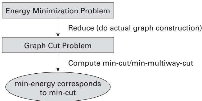
Figure 38.1 Schematic of the graph cut technique. Here, the cuts are labelings and the cost of a cut represents the energy. Credit: Chittu Tripathy and Bruce Donald.
38.4.1 Using Graph Cuts in Energy Minimization
A standard form of energy function is given by
where defines the neighborhood system of interaction, denotes the assignment cost function, and is the separation cost function. This energy function was studied extensively in computer vision and the graph cut technique has been applied successfully to minimize such energy functions.
The general idea behind the graph cut technique is to construct a specialized graph for the energy function to be minimized, so that minimization of energy (locally or globally) corresponds to computing a minimum cut of the graph. Figure 38.1 illustrates the general framework for energy minimization using graph cuts.
38.5 Representation of Energy Functions by Graphs
Graph Representable Functions A function of binary variables is graph representable if there exists a graph with terminal vertices and and a subset of vertices such that, for any configuration , the value of the energy is equal to a constant plus the cost of the minimum - -cut among all cuts in which , if , and , if (). We say that is exactly represented by if this constant is zero.
Note that the addition of a constant does not change the minimum energy configuration.
This definition leads to the following result. If the energy function is graph representable by a graph and a subset , then it is possible to find the exact minimum of in polynomial time by computing the minimum - -cut on .
Two important classes of energy functions called and in terms of graph representability are discussed in the following sections, which provide general procedures to construct graphs.
The Class
The class is a subset of energy functions where each individual term can be expressed as a function of at most two Boolean variables.
Theorem 38.1 ( Theorem) Let be a function of binary variables from the class , i.e.,
Then is graph representable if and only if each term satisfies the following condition, called the regularity condition:
Note that functions of one Boolean variable are always regular.
Graph Construction for
Construct a graph as follows:
- The vertex set , where encodes the Boolean variable , such that if , and if .
- We write to mean an edge with the weight if or an edge with the weight if .
- For each term , add an edge . Refer to figure 38.2 a and b.
- As figure 38.2 c, d, and e shows, for each term
add the following three edges:
- ,
- , and
- with weight . The function is called the functional, which we formally define in section 38.7. Note that for regular functions of two variables, .
- Once the graph for each individual term is constructed, merge the graphs together to get the final graph. The merging is justified by the additivity theorem, which states that the sum of two graph representable functions is graph representable.
Each edge weight is made nonnegative by construction, which is important since we construct the graph to finally compute a min-cut of the graph.
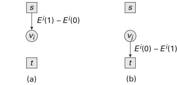
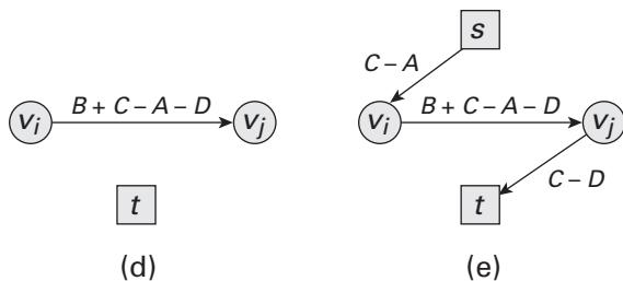
Figure 38.2 Graph cuts for functions . (a) Shows the graphs for where ; (b) shows the graphs for where ; in (c), the table shows the individual terms for the two variable function ; in (d) we show the third edge for ; (e) represents the complete graph for when and . Note that (e) shows one of the four possibilities [2].
NP-Hardness of General Functions
Theorem 38.2 Let represent an energy function of two variables that is not regular. Then, minimization of functions of the form
where are arbitrary functions of one variable and , is NP-hard.
The Class
Theorem 38.3 ( Theorem) Let be a function of binary variables from the class , that is,
Then is graph representable if and only if is regular.
The regularity condition in case of functions of three Boolean variables will be stated after introducing a few more concepts. We define the functional of an energy function to be a mapping from the set of all functions of Boolean variables to the set of all real numbers given by the following equation:
For example, for a two variable function . The functional is linear, i.e., .
For a three-variable function we compute the functional as follows. We take all projections of two variables of (a projection means fixing the value of one variable and then computing , which can now be thought of as a function of two variables) with positive values of functional . If we don’t find such a projection, then is regular.
Graph Construction for
Construct a graph as follows:
- The vertex set , where encodes the Boolean variable , such that if , and if .
- We write to mean an edge with the weight if or an edge with the weight if .
- For the terms in the forms and , the edges are added as explained in the construction of the graph for . Refer to figure 38.2. We now construct the part of the graph where each term involves three Boolean variables, that is, the terms of the form .
- For each term
, add one extra vertex
in addition to the vertices
and
. If
, then the following edges are added (see figure 38.3 b):
- ,
- ,
- ,
- with weight ,
- with weight ,
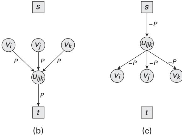
Figure 38.3 Graph cuts for functions . (a) Shows the terms depending on three variables . Here . (b) Represents the graph for the case when . (c) Shows the graph for the case when [2].
- with weight , and
- with weight .
If then we add the following edges (see figure 38.3 c):
- ,
- ,
- ,
- with weight ,
- with weight ,
- with weight , and
- with weight .
- Once the graphs for each individual term is constructed, merge the graphs together to get the final graph. The merging is justified by the additivity theorem.
Comments
The graph construction technique used for the class of functions in does not introduce any additional vertices in beyond necessity, and in the case of functions in the class , only one extra vertex for every ternary interaction term is introduced. This construction yields much smaller graphs and hence the minimum cut can be computed efficiently.
The graph cut technique using the above graph construction procedure is very powerful when applied to stereo and multicamera scene reconstruction. The usefulness of the technique is strongly supported by the experimental results.
Since , the class includes a larger class of functions that can be minimized using the graph cut framework.
Finally, it will be interesting to see how the graph cut technique can be applied in other areas of computational biology and molecular biophysics.
Exercise Are the pairwise energy functions commonly used for protein design in class or ? Compare and contrast both classes of functions, to those used in protein design.
Exercise Can you use graph cuts to model side-chain rotamer assignments, and thereby devise an efficient algorithm for computing the GMEC?
Exercise Can you use graph cuts to model NMR resonance assignments, and thereby devise an efficient algorithm for structure-based assignment?
References
[1] Ramin Zabih and Vladimir Kolmogorov. Spatially coherent clustering using graph cuts. Proceedings of IEEE Conference on Computer Vision and Pattern Recognition (CVPR) 2, (2004):437–444.
[2] Vladimir Kolmogorov and Ramin Zabih. What energy functions can be minimized via graph cuts?. IEEE Transactions on Pattern Analysis and Machine Intelligent, 26;2(2004):147–159.