Chapter 45CS-Rosetta: Protein Structure Generation from NMR Chemical Shift Data
This chapter describes a version of the Rosetta protocol for structure prediction [1]. Rosetta has been used in protein structure prediction and design, and in the design of protein:ligand interactions.
Introduction
Modern technological advances have expedited the determination of protein structures. For example, NMR spectroscopy provides experimentalists with restraints, such as NOEs and RDCs, to calculate the structure of a molecule. Some programs such as CYANA and DYANA take experimentally measured NOEs as input, and use simulated annealing and simplified molecular dynamics to compute a structure. However, the experiments to measure NOEs are time-consuming and can be expensive, and it is also sometimes challenging to assign the NOEs. Indeed, robust algorithms for automated NOE assignment are an active area of research in NMR methods development (chapters 8, 14, 17.4, 18, and 33).
Other scientists have developed techniques that predict protein structure, using less experimental information than traditional NMR protocols. One such strategy starts with the protein sequence information and uses empirical molecular mechanics energy functions and computational biophysics, plus information from a library of previously determined structures, together with statistical information about backbone and rotamer conformations. It would be incorrect to say these approaches do not use empirical data, since the weights and nuisance parameters in the energy functions and employed by the algorithm have been fit to these other, previously determined empirical structures. But they do not use experimental data measured on the particular protein for which a structure is being predicted. In this sense, it would be fair to view such approaches from a point of view including statistical parameter estimation or machine learning. Thus, the scoring function and even the algorithm is constructed using a training set of data and structures, and is then demonstrated on a (usually disjoint) testing set of structure prediction problems. In these early days of computational structural biology, issues of convergence, statistical bias, undersampling, and overfitting are also starting to receive attention. Finally, Rosetta relies critically on a library of fragments from a curated database of protein structures. Rosetta may be viewed as a stochastic algorithm combining local homology fitting, energy minimization, and random sampling. This having been said, the Rosetta suite of software is large and complex; this chapter only touches on a few of its concepts.
The Rosetta protocol employs classical Monte Carlo sampling plus a database search strategy to attempt to produce a likely protein fold, without using empirical restraint data (e.g., NOEs) for the protein. Rosetta has been one of the most successful blind-prediction programs, and the authors of CS-Rosetta augmented the basic Rosetta program to use NMR chemical shifts (CS) in an attempt to increase accuracy.
Rosetta
Rosetta is a protein structure prediction program, that starts with the primary sequence and searches conformation space to find a global fold. Given the sequence of a protein, Rosetta predicts protein structure via database search and comparison, combined with modeling energy minimization. Rosetta uses a Monte Carlo simulated annealing procedure. In this chapter we will distinguish vanilla Rosetta (which does not use experimental data) from CS-Rosetta (which uses experimentally measured NMR chemical shifts). “CS” stands for “chemical shifts.”
Monte Carlo Procedure Monte Carlo is a random-walk-based exploration of the search space. Rosetta uses simulated annealing, an algorithm that randomly explores neighboring conformations using a simulated Boltzmann distribution until it converges to some point in the search space. The simulated annealing algorithm in general has three phases: generation, acceptance, and update. The generation phase is the phase in which a new configuration is randomly selected from neighboring points in the search space. Some values of the configuration are modified slightly, and the new configuration is returned. The acceptance phase accepts a configuration generated by the generation phase if it is of lower overall energy; if a configuration is of higher energy than the current configuration, the move is accepted probabilistically depending on the energy difference and a parameter, , commonly “temperature.” In the update stage, is modified based on the current configuration’s energy and as some function of time. A function mapping configurations and times to values for is called an annealing schedule. There exists some annealing schedule, such that the search will converge as time goes to infinity. However, finding this schedule is NP-hard.
Correctness and Time Bounds Probabilistically, the Monte Carlo procedure is expected to identify the globally optimal solution as rapidly as brute force search: If there are total possible states , and . In practice, brute force search often suffers from the curse of dimensionality, and with simulated annealing the possibility of identifying the optimal solution without covering the full combinatoric search space becomes nonnegligible. Fabio Romeo and Alberto Sangiovanni-Vincentelli proved that the probability of identifying the optimal solution goes to 1 as time goes to infinity, but this proof offers little insight into the behavior of the algorithm given finite time constraints [2]. The model of finite time and space, and asking what can an algorithm compute in a finite time bound whose value is some function of the input size (e.g., polynomial or exponential), models a computer’s efficiency to solve the problem.
General Applicability Simulated annealing (SA) has the potential to find the optimal solution in subexponential time. However, it’s not clear if it will run faster than brute force search. It’s not even clear how close the answer returned by SA is to the right answer. Understandably, for polynomial time solvable problems, such as classical search and sort, this is an unreasonably loose bound on performance, and deterministic algorithms are preferred. In NP-complete cases, however, ease of programming and potential success rate continue to make simulated annealing a popular strategy.
CS-Rosetta
Shen et al. [1] use SPARTA, also created by their lab, to build a fragment library from which Rosetta draws for fragment replacement. After the fragment library is generated for the protein sequence, traditional Rosetta is run to generate candidate structures. In summary, the CS-Rosetta structure determination proceeds as follows:
- Fragment Library Generation CS-Rosetta employs SPARTA, which is an algorithm for chemical shift back-calculation trained on 200 proteins, to select from the 5,665-protein structural database a library of protein fragments that best fit the chemical shifts observed from experimental data, fit via molecular fragment replacement (MFR; see chapter 17.2) [3]. This fragment library is fed into traditional Rosetta.
- Fragment Replacement Fragment replacement begins with an uncoiled peptide strand. Random 9-residue windows are selected by Rosetta, and the fragment library from the previous step is searched for the 25 best matches ranked by sequence similarity and conformational energy. A random match is selected from the 25 and the backbone angles of the protein are modified to match the fragment. This proceeds until all residues have been assigned, and up to 2,000 iterations past that point. As in all other parts of the procedure, the change is accepted if the resulting structure has lower energy, and accepted according to the simulated annealing Metropolis criterion if higher.
- Side-Chain Minimization Side-chains are computed in CS-Rosetta (and traditional Rosetta) by randomly selecting a residue, randomly assigning a rotamer, and keeping that assignment according to the simulated annealing Metropolis criterion.
- All-Atom Minimization After sufficient iterations of side-chain minimization have been completed, CS-Rosetta randomly selects an atom and perturbs it randomly, and minimizes the whole protein to accommodate the perturbation. Again, SA procedures are observed to encourage the program to travel into the global and not the local minimum.
5. Termination The program was assumed to have converged when the next lowest energy conformation generated was less than 2 Å RMSD from the current best, and the structure accepted. 10,000 to 20,000 all-atom models were generated for each protein.
Computational Experiments Performed Shen et al. ran CS-Rosetta on 16 small proteins whose structure was known at the time of the experiment and performed 9 additional blind structure predictions. They also compared accuracy of SPARTA to DC, an alternative algorithm, and compared the accuracy of models generated.
Results
Even though SPARTA was only 10% more accurate than DC, the fragments selected were significantly more accurate for Rosetta’s MFR procedure. When using DC instead of SPARTA, the backbone coordinate error obtained for fragments selected from the structure database is 25%–65% higher than those for the respective SPARTA-assigned database. Rosetta does not account for chemical shift data when performing side-chain prediction and minimization, which resulted in some deviation from the native structure, and, interestingly, the “goodness” of the structure. For the 9 unknown structures, CS-Rosetta performed well in the ordered regions, deviating no
Table 45.1 Accuracy of CS-Rosetta structures for 16 proteins
| Protein Name | PDB ID | RMSD bb , Å | RMSD all , Å | |||
|---|---|---|---|---|---|---|
| GB3 | 2OED | 14/26 | 56 | 332 | 0.69 | 1.40 |
| CspA | 1MJC | 0/33 | 70 | 405 | 1.57 | 2.19 |
| Calbindin | 4ICB | 47/0 | 75 | 435 | 1.20 | 2.01 |
| Ubiquitin | 1D3Z | 18/25 | 76 | 426 | 0.75 | 1.35 |
| XcR50 | 1TTZ | 28/16 | 76 | 352 | 1.53 | 2.30 |
| DinI | 1GHH | 36/21 | 81 | 463 | 1.76 | 2.29 |
| HPr | 1POH | 29/23 | 85 | 419 | 1.01 | 1.79 |
| MrR16 | 1YWX | 23/35 | 88 | 514 | 1.52 | 2.28 |
| TM1112 | 1O5U | 10/52 | 89 | 524 | 1.51 | 2.22 |
| PHS018 | 2GLW | 20/41 | 92 | 531 | 1.28 | 2.08 |
| HR2106 | 2HZ5 | 37/25 | 96 | 470 | 1.65 | 2.42 |
| TM1442 | 1SBO | 41/23 | 110 | 647 | 1.09 | 1.88 |
| Vc0424 | 1NXI | 55/25 | 114 | 679 | 1.72 | 2.51 |
| Spo0F | 1SRR | 55/25 | 121 | 590 | 1.24 | 2.02 |
| Profilin | 1PRQ | 41/41 | 125 | 595 | 1.71 | 2.34 |
| Apo_lfabp | 1LFO | 15/70 | 129 | 688 | 1.64 | 2.18 |
Note: Running CS-Rosetta on the 16 known structures, predicted structures were no more than 2.5 Å RMSD from the native conformation. Reprinted from [1].
more than 2 Å from the native structure, and no more than 1 Å RMSD for 6 of the 9 proteins. In the disordered regions, CS-Rosetta was less able to produce native conformations. This is explained by the nature of Rosetta’s scoring function, which favors hydrogen bonds and therefore extended the protein’s secondary structure a few residues beyond the native structure. This could be alleviated by flagging the loops of the protein, which can be identified via Random Coil Index (RCI), and this improved accuracy further in the ordered sections. Additionally, the protocol DP (DP score) was used to score experimentally derived structures and CS-Rosetta predicted structures, and DP scored the experimentally derived structures 10–40% higher, mostly on account of differences in core side-chain packing. Recall that DP score (“Discriminating Power”) was introduced in chapter 33.
Chemical shift data, measured in parts per million, are among the most exquisitely sensitive NMR data to the local electronic environment of a nucleus. The results of CS-Rosetta (table 45.1, figures 45.1, 45.2, plates 47, 48) show that there is a computational protocol to determine structures from these data alone. This is significant, since CS data is currently the cheapest NMR data to record. Note that the CS-Rosetta protocol requires the resonances (chemical shifts) to be assigned.
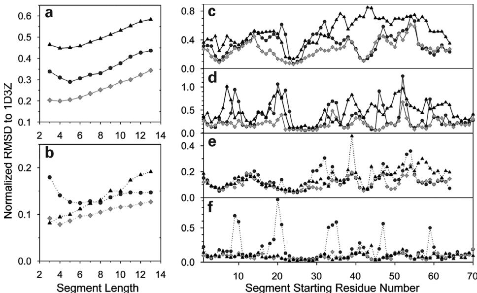
Figure 45.1 (plate 47) Plots of normalized accuracy of database fragments selected for ubiquitin. For each ubiquitin segment, 200 fragment candidates of the same length were selected using either the standard Rosetta procedure (filled triangles), or an MFR search of the 5,665-protein structural database, assigned by the programs DC (filled circles) or SPARTA (filled diamonds). For all panels, coordinate RMSDS (N, , and ) between query segment and selected fragments are normalized with respect to randomly selected fragments. (a and b) Average (a) and lowest (b) normalized RMSD of 200 selected fragments, as a function of fragment size, relative to the X-ray coordinates of the corresponding ubiquitin segment, averaged over all (overlapped) consecutive segments. (c and d) Average normalized RMSD of 200 nine-residue (c) and three-residue (d) fragments relative to the X-ray coordinates, as a function of position in the ubiquitin sequence. (e and f) Lowest normalized RMSD of any of these selected nine-residue (e) or three-residue (f) fragments. Reprinted from [1]. Copyright 2008 National Academy of Sciences.
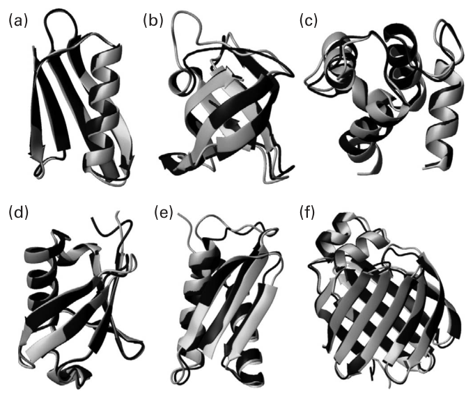
Figure 45.2 (plate 48) Six structures generated by CS-Rosetta; the ordered secondary structure is very similar but the loops differ significantly between experimental and predicted structures. Backbone ribbon representations of the lowest-energy CS-Rosetta structure (red) superimposed on the experimental X-ray/NMR structures (blue), with superposition optimized for ordered residues. (a) GB3, (b) CspA, (c) calbindin, (d) ubiquitin, (e) DinI, (f) Apo_lafbp. Reprinted from [1].
References
- [1] Yang Shen, Oliver Lange, Frank Delaglio, Paolo Rossi, James M. Aramini, Gaohua Liu, et al. Consistent blind protein structure generation from NMR chemical shift data. Proceedings of the National Academy of Sciences 105;12 (2008): 4685–4690.
- [2] D. Mitra, F. Romeo, and A. S. Vincentelli. Convergence and finite-time behavior of simulated annealing. Advances in Applied Probability (Sept 1986).
- [3] G. Kontaxis, F. Delaglio and A. Bax. Molecular fragment replacement approach to protein structure determination by chemical shift and dipolar homology database mining. Methods in Enzymology 394 (2005):42–78.