Chapter 1Introduction to Protein Structure and NMR
This chapter presents the basics of protein structure, and then discusses some principles in protein structure determination by nuclear magnetic resonance (NMR). We will use these basic facts about proteins and the NMR technique in developing several algorithms and computational frameworks in this book.
This first chapter introduces and ties together the concepts of protein kinematics, experimental data for geometric restraints, and sophisticated algorithms to determine structures given restraint data. We begin with simple examples, to illustrate the general principles that will be investigated in depth in this book.
Protein Structure
Proteins are linear polymers of amino acids, and different sequences of amino acids generally have different three-dimensional protein structures. Figure 1.1 shows the cartoon structure of a prototypical amino acid, where R stands for any of 20 natural amino acid side-chains.
There are two important exceptions. The glycine side-chain is simply a single hydrogen atom bonded to the , and so effectively glycine has two atoms. Thus, glycine has exceptional conformational flexibility compared to the other amino acids. Proline is the only cyclic amino acid.
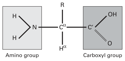
Figure 1.1 The structure of a typical amino acid.
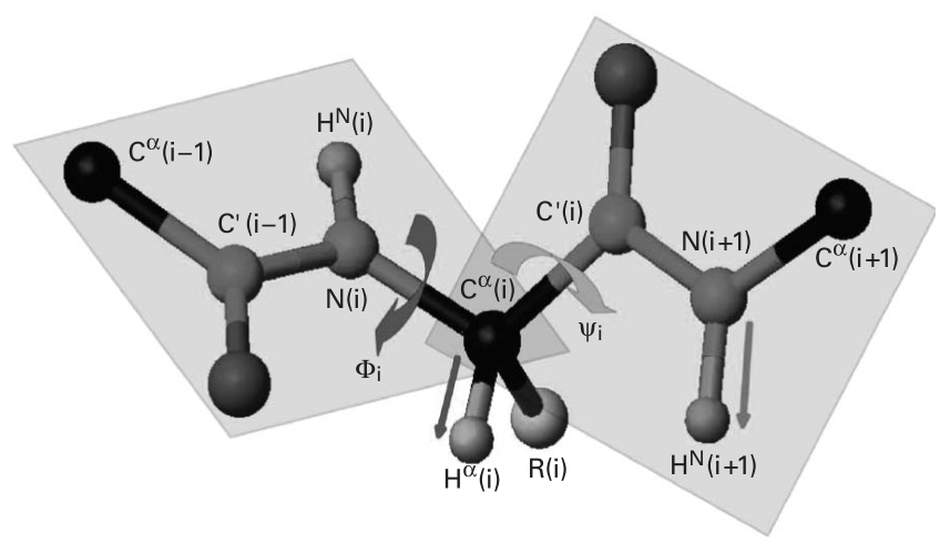
Figure 1.2 (plate 1) The and torsion angles of peptide backbones.
The cyclic structure of proline’s side-chain restricts its backbone dihedral angle to approximately degrees, giving proline more conformational rigidity than other amino acids.
Sometimes will be written as . The carbonyl carbon is often written as , and the protons bonded to and N, respectively, are written as and .
Through a reaction of the corresponding amino and carboxyl groups, amino acids form peptide bonds. We refer to the N, , O, and atoms in the peptide as the peptide backbone. The characteristics of the peptide bond is shown in figure 1.2 (plate 1). The peptide bond is ideally, although not in reality, planar and rigid, and the rotation is only allowed by the () and () torsion angles. Given a sequence of amino acids, we are interested in finding all torsion angles () for all peptide units to determine the three-dimensional structure of the protein backbone. In some models the atom is considered with the backbone (chapter 11), which requires handling glycine and proline as special cases.
Structure Determination of Proteins with NMR Spectroscopy
At a high level, some NMR spectra can give us some biophysical (frequency) signals, which encode geometric information about the protein structure, such as the distance and angle information. Determination of the three-dimensional structure ( and angles) of the protein backbone can be regarded as a graph realization or distance geometry problem, using measured distance or angle constraints. This problem can be solved easily if the exact distance constraints between all pairs of atoms are known. However, the NMR data unavoidably is uncertain and may have missing data. In fact, the noise in NMR spectra increases the complexity of our computational task. Finally, in general, distances can only be measured between pairs of protons less than 6 Å apart.
Nuclear Overhauser Enhancement (NOE) The NOE is a consequence of dipole-dipole coupling and cross-relaxation between different nuclear spins [1], and is used to measure the distance between atoms (usually protons) in proteins. The relation between the observed NOE intensity and the distance is ideally .
NMR Assignment Problem The NMR resonance assignment problem is to find the mapping from each observed frequency (resonance) in NMR spectra to each NMR-active nucleus in the protein. More precisely, let denote the set of atoms, and denote the set of observed resonances. Physics defines a function (which we cannot write down precisely), . We have the inverse problem: to compute , where is called the assignment. We will discuss the resonance assignment problem in later lectures.
Distance Geometry Problem Let where denote the (3D) coordinates for atoms in the protein structure. We can represent all by a matrix, called the distance matrix, where each item intercrossed at the th row and the th column corresponds to . Now, the distance geometry problem is to find coordinates1 such that the distance constraints in the given distance matrix are all satisfied. We classify the distance geometry problem into several cases according to different kinds of distance matrices:
- Problem with All Exact Distances If the exact distances between all pairs of atoms are known, the problem can be solved in time by using the Singular Value Decomposition method, where denotes the number of atoms. More recently, Dong and Wu [2] have shown that this problem can be solved in linear time by using a “Geometric Build-Up” algorithm.
- Problem with Sparse Sets of Distances Given only a subset of the distances, the distance geometry problem becomes difficult to solve. Saxe [3] has shown that this problem is (strongly) NP-hard.
- Problem with All Distances But with Some Errors This problem has been examined by Berger, Kleinberg, and Leighton [5]. They mainly considered the approximation solution of this problem.
- Problem with Interval Bounds of Distances Because of the noise from experimental data, we may only get some lower and upper bounds on the distances. It has been demonstrated that such a problem is still hard to solve. More and Wu [4] considered the -approximation2 of this problem. They showed that if is smaller than a certain value, finding an -optimal solution to the distance geometry problem is still NP-hard.
1 Using kinematics, the coordinates are related to the and angles in the conformation of the protein backbone.
2 The solution is called -optimal if distance errors in the solution are within a tolerance of .
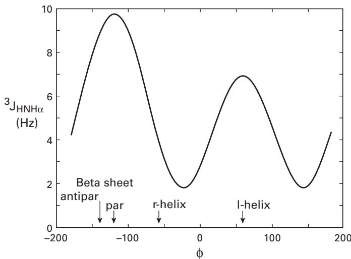
Figure 1.3 The Karplus relationship between the three-bond coupling constant and the torsional angle . Credit: http://www.cryst.bbk.ac.uk/PPS.
Later chapters in this book will describe upper and lower bounds for distance geometry problems.
Scalar (Spin-Spin) Coupling Constant The 3-bond scalar coupling constant provides a measurement of torsion angle information, which is different in different kinds of regular secondary structures, such as helix and sheet. The correspondence between and can be found from the empirically derived Karplus curve, as shown in figure 1.3. More specifically, the following values of in some regular secondary structures are obtained [1]:
- Right-handed alpha helix, , Hz
- Right handed 3.10 helix, , Hz
- Antiparallel beta sheet, , Hz
- Parallel beta sheet, , Hz
- Left-handed alpha helix, , Hz
The preceding data provide a method for identifying regular secondary structures based on the measurements of .
The reader may wonder, if our goal is to compute and angles, why not measure them directly using scalar couplings? There are four reasons. (1) The relationship between and is multivalued (figure 1.3), necessitating a logical “OR” approach and a tree-search. (2) The data are uncertain and noisy, and generally only provide loose bounds on dihedral orientations. (3) Higher-resolution structures are possible by combining different NMR data. Nevertheless, scalar couplings provide valuable geometric measurements when they can be recorded. Finally, (4) these experiments are much less sensitive for large proteins, compared to other NMR measurements.
References
- [1] Kurt Wuthrich. NMR of Proteins and Nucleic Acids. New York: John Wiley & Sons, 1986.
- [2] Q. Dong and Z. Wu. A linear-time algorithm for solving the molecular distance geometry problem with exact inter-atomic distances. Journal of Global Optimization, 22 2002: 365–375.
- [3] J. B. Saxe. Embeddability of weighted graphs in -space is strongly NP-hard. Proceedings of the 17th Allerton Conference on Communications, Control, and Computing, 1979, 480–489.
- [4] Jorge More and Zhijun Wu. -Optimal solutions to distance geometry problems via global continuation, in P. M. Pardalos, D. Shalloway, and G. Xue (eds.,). Global Minimization of Nonconvex Energy Functions: Molecular Conformation and Protein Folding. pp. 151–168, American Mathematical Society, 1996.
- [5] Bonnie Berger, Jon Kleinberg, and Tom Leighton. Reconstructing a three-dimensional model with arbitrary errors. Journal of the ACM (JACM), 46(2) 1999: 212–235.