Chapter 4MBM, SVD, PCA, and RDCs
In this chapter, we review the basic ideas of maximum bipartite matching (MBM), singular value decomposition (SVD), principal component analysis (PCA), and residual dipolar coupling (RDC) geometry. These algorithms are useful in computational biology in general, and structural biology and molecular biophysics in particular, and will be used in several applications in this book.
Each of these topics could be covered in some depth and breadth, even requiring several lectures. It is useful to have the basic primer on these techniques in one short chapter here. Later, we will explore details and applications of these fundamental concepts.
MBM
The input of an MBM problem is a complete bipartite graph with a weight function , such that , , and . More generally, , but we can add edges with weight 0 to the graph to make it complete bipartite. Here, can be visualized as the set of vertices on the left, and as the set of vertices on the right.
A matching is a set of nonintersecting edges. The output of MBM is a matching between and with the highest weight. That is,
Example 4.1 In the assignment problem, we want to match the residues in the model with the peaks observed in HSQC. This problem is modeled as an MBM problem as follows:
- Let , .
- For any , , let
Here is the actual RDC data obtained from experiments, and is the simulated RDC data back-calculated from the model.
The Hopcroft–Karp algorithm finds the maximum bipartite matching in time [1, 2].
An MBM problem can be very sensitive to noise, as shown in the following example.
Example 4.2 Let , , the ground truth weight is , , , . Then, the maximum matching is . However, if there is a noise on the weight of the edge such that the weight we observed is 11, then the maximum matching will become , which does not share any edge with the ground truth.
SVD
Definition
SVD is a technique to decompose a matrix into the product of three matrices. For any -by- matrix , there exists a decomposition of to the product of three matrices such that
- is an unitary matrix, that is, where is the identity matrix.
- is a diagonal matrix, which means that all the entries outside the main diagonal of are zero. Thus, , , .
- is the transpose of a unitary -by- matrix .
Properties
One of the most important properties of SVD is that it can be used to calculate the best solution to a linear system that minimizes the least-square norm. The problem is defined as follows:
Problem 4.1 Let be an matrix, and be an vector. Find an vector that minimizes , where , is the th component of , etc. That is
can be calculated as follows by applying SVD to .
- Calculate the SVD of . Let , where . Let be an diagonal matrix.
- Let be the pseudoinverse of .
- Let .
It can be proved that is the minimal-norm least-square solution to .
When is symmetric (), and positive semidefinite (that is, for any vector , ), then and the are the eigenvalues of .
PCA
PCA is a technique to reduce the dimension of high-dimensional data, in order to simplify the analysis. PCA is an orthogonal linear transformation that transforms the data set to another coordinate system such that the distance variance among data is mainly in the first several dimensions. PCA is useful because in many real-life instances, we do not know the structure of the problem, so we have to model the data in a very high-dimensional space. However, the data set itself has some underlying structure such that the variance of data can be approximately characterized in a space of much lower dimension. For example, imagine a case where, in , all of the data are generated approximately in a line (1-dimensional space). Then PCA can find a new coordinate system such that this line is the first coordinate (also known as the first principal component). To analyze the distance between points in the data set, we do not need to consider the remaining 99 dimensions.
Calculating PCA by SVD
Let be an matrix, in which each column is a data vector in . Without loss of generality, we assume that has zero empirical mean, that is, .
To find the subspace that best represents the variance of , let be the covariance. Then, compute the SVD for . Notice that is symmetric and positive semidefinite, so the SVD of must be , where the diagonal of consists of all the eigenvalues of , and the column vectors of are the normalized eigenvectors (recall that is the normalized eigenvector of an eigenvalue of , if and ). Then, we choose the largest eigenvalue eigenvectors as the axes to project on. Without loss of generality, suppose are the largest eigenvalues of , and let be their eigenvectors, respectively. Then, is the transformation matrix, and is the projection of the original data vector to a -dimensional subspace that best represents the variance of the data in .
RDCs
NOEs provides interproton distance information for a protein. However, such information is only available when the distance between two nuclei is short (under 6 Å). RDCs, on the other hand, can provide global structural information between spins even when the distance between them is very large.
Definition 4.1 The residual dipolar coupling between two spins and , is defined as follows:
where is the Planck’s constant, is the gyromagnetic ratio, is the interspin distance, is the angle between the interspin vector and the external magnetic field (see figure 3.5). In NMR, spins and are sometimes called and (see figure 4.1).
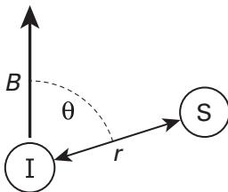
Figure 4.1For example, in NVR, RDC is used to measure the orientation of the NH bond vector for each residue (chapter 14). Therefore, the distance in (eq. 4.1) is known. In this case the RDC measures the global orientation of the NH bond.
Exercise How can SVD be used to analyze RDC data? What is the relationship between this use of SVD, and the PCA method?
References
- [1] John E. Hopcroft and Richard M. Karp. An Algorithm for Maximum Matchings in Bipartite Graphs. SIAM Journal of Computing 2(4) (1973): 225–231.
- [2] Thomas H. Cormen, Charles E. Leiserson, Ronald L. Rivest, and Clifford Stein. Introduction to Algorithms, 2nd ed. Cambridge, MA: MIT Press, pp. 696–697.