Chapter 5Principal Components Analysis, Residual Dipolar Couplings, and Their Relationship in NMR Structural Biology
Anthony K. Yan and Bruce R. Donald
In biochemistry, nuclear magnetic resonance (NMR) is a powerful tool for analyzing the structure and dynamics of proteins in solution. Recently, research has taken advantage of a type of NMR data known as residual dipolar couplings (RDC). The physics of RDC’s tells us they are formed from a time and ensemble average. This ensemble average is mathematically similar to the data analysis technique known as principal components analysis (PCA). In this chapter, we consider the formal relationship between the two, and consider the information content of the RDC formalism with respect to protein flexibility. After mastering this chapter, you will understand the fundamentals of RDCs, which are important in structural biology, and know the foundations of PCA, one of the most important algorithms in computational science and applied statistics.
In classical physics (or molecular dynamics, MD), ensemble averages are over continuous degrees of freedom. To keep the discussion simple for our broad audience, in this chapter we pretend that the ensembles are discrete. By way of intuition, in quantum mechanics the ensemble is discretized, so our derivation is analogous to averaging over quantum states.
At any rate, the reader who is familiar with continuous probability distributions and Jacobians will find it easy to generalize all the math in this chapter to continuous ensembles. Basically, the key ideas in the lecture are very simple, and we didn’t want to have intimidating integrals everywhere: This is why we feel that discrete averages make for a cleaner presentation.
Introduction
Residual dipolar couplings (RDCs) are a type of data from NMR that has been useful for solving protein structures and solving the assignment problem. According to the physics of RDCs, they are based on the relationship between internuclear vectors and a set of parameters known as the Saupe alignment tensor.
In this chapter, we consider the relationship between the Saupe alignment tensor and a data analysis technique known as principal components analysis (PCA). It turns out that the Saupe matrix is mathematically similar to the covariance matrix in PCA. The Saupe matrix is the result of an ensemble average of internuclear vectors, and contains statistical information about the ensemble that is very similar to the statistical information contained in PCA.
Intuitively, PCA gives us the spread or variance of a set of points along the principal axes of the ellipsoid that best fits the point set. One might have hoped that the Saupe matrix would contain exactly the same information as PCA. However, this is not the case. Instead, the Saupe matrix contains an upper bound of the variances of its ensemble. It will be shown that the Saupe matrix along with the ensemble average contains information precisely equal to PCA. However, the ensemble average is not contained within the RDC data; consequently, we are able to compute only an upper bound on the ensemble’s variances. If the average of the ensemble were estimated by alternative means, we could use the Saupe matrix to perform PCA on the ensemble.
Below, we derive PCA, and explain its properties. Although this may be a review to some readers, it is useful for the exposition here as we will also derive the Saupe matrix formalism and explain its relationship to the derivation of PCA.
The structure of this chapter is as follows. First we derive PCA in section 2. In section 3, we derive the Saupe alignment tensor. In section 4, we compare the Saupe matrix to PCA, and explain their relationship. Finally, in section 5, we discuss future work and possible applications. In the appendix, we explain how to efficiently perform PCA on data sets with very large dimension and a relatively small number of data points.
Introduction to PCA
We motivate PCA by considering the statistics of discrete sets of . Let , where and . The standard statistical characterizations of are the mean and variance (standard deviation):
Very often, our data is not in , but instead is in . We would like to define the direct analogs of mean and standard deviation in higher dimensions. Consider a point set in . Let , where and . The mean is easy to define:
The analog of the standard deviation is less easy to define in . However, we can simplify things by projecting our data points onto a one-dimensional line. We will then compute the directional variance along the line.
To simplify our presentation, let us assume that our data has already been zero-meaned:
We project onto a line through the origin, which is specified by the unit vector . Let be the projection of onto the line specified by :
where is the (signed) length of along the line specified by . We can now compute the average and variance of the . The mean is zero:
since we assume the are zero-meaned.
Now let’s compute the directional variance, which we define as follows:
Definition 5.1 If , then the directional variance along unit vector is
Playing with algebra, we have:
So we have,
The term is the outer product of with itself and is an matrix. It is not to be confused with , which is the inner product of with itself, which is a scalar. If is zero-meaned, then is known as the covariance matrix of . For this chapter, we shall say that if is arbitrary (not zero-meaned), then is the pseudo covariance matrix of . The pseudo covariance matrix equals the covariance matrix when is zero-meaned. Later on, we shall be forced to consider the relationship between pseudo covariance matrices and true covariance matrices.
Let’s pause now to consider where we are. Given , we can compute the covariance matrix . Equation (5.11) tells us that given the covariance matrix, we know the directional variance for all directions . Intuitively, is a complete description of the variance of in .
Now that we have a notion of standard deviation in , we should study its geometric properties. First notice that is symmetric by construction. This means has real eigenvalues and orthogonal eigenvectors. Furthermore, we know that is positive semidefinite because for all unit vectors . This is because each term of the sum in equation (5.8) is non-negative. Consequently, has non-negative eigenvalues.
Let be eigenvectors of with eigenvalues :
where is the Kronecker delta. In short, is our favorite kind of matrix (orthogonal eigenvectors, non-negative eigenvalues).
We now consider the geometry associated with . We’ll consider two aspects of . First, we’ll make a plot of the directional standard deviation and second, we’ll consider the shape of the associated Gaussian distribution in .
Definition 5.2 If , then the directional standard deviation along unit vector is just the square root of the directional variance:
One can imagine plotting the directional standard deviation for all directions. One would do this by plotting all the points for all unit vectors . Intuitively, this is a polar plot where, instead of using angles to specify a direction, one uses a unit vector. The radius of the plotted point is the directional standard deviation. For an illustration of this, see figure 5.1, which is a plot in . If the eigenvalues of the covariance matrix are all identically equal, then the directional standard deviation is isotropic, hence our plot is circular. On the other hand, if the eigenvalues are not equal to each other, then the plot has a lobes and a dimpled structure. Perhaps surprisingly, the plot is not an ellipsoid, but might more aptly be called a “dimpleoid.”
Next, we consider the Gaussian distribution, which is associated with the covariance matrix. We would like to know the shape of a Gaussian distribution which has the same directional standard deviations as our covariance matrix. Let be our covariance matrix. Let be a zero-meaned Gaussian with covariance matrix . It can be shown that the directional standard deviations of are equal to the directional standard deviations of . The directional standard deviation of a probability distribution in is computed from its covariance matrix, which is the expected value (average) of the outer product:
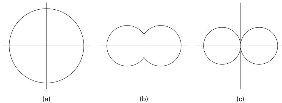
Figure 5.1 Examples of directional standard deviations in . In these three examples, we make polar plots of the directional standard deviation for three different covariance matrices. All three plots are in the Principal Order Frame (POF) of the covariance matrix, so that the eigenvectors are along the and axes. In (a) the eigenvalues are equal. In (b) the eigenvalues are not equal and nonzero, with the eigenvalue being smaller than the eigenvalue. In (c) the eigenvalue is zero. Credit: Bruce Donald and Anthony Yan.
where the integral is over , is a volume element of , and is a probability distribution over . We have abused notation in equation (5.19) since is a probability distribution, not a set of points.
To make things simple, let’s work in the POF of the covariance matrix. In the POF, is diagonal, and so is its inverse . It is now easy to write down explicitly:
The probability distribution can be visualized by its level sets. In particular, let’s consider the level set that occurs when the exponent is equal to unity. In this case, we have the set of all that satisfies . If we write this explicitly in the POF, we get
where is the th component of in the POF; is the eigenvalue associated with the eigenvector pointing along the th coordinate axis (and is associated with the component ). Recall that in the POF, the eigenvectors are along the coordinate axes.
The level set represented by equation (5.23) is easily recognized as the equation for a hyper-ellipsoid with semiaxes . The length of the semiaxes are equal to the directional standard deviation along the semiaxes, and are also the standard deviations of the Gaussian distribution (see figure 5.2).
However, for directions not along an eigenvector, the ellipsoid’s radius is not equal to the directional standard deviation. To illustrate this point, see figure 5.3, which overlays the level set of the Gaussian with its directional standard deviation.
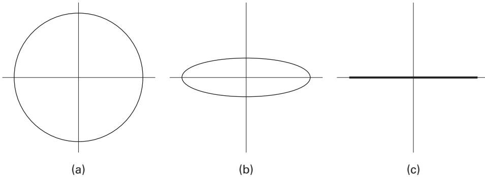
Figure 5.2 Examples of Gaussian ellipsoids in . In these three examples, we make polar plots of the level sets for three Gaussians associated with three different covariance matrices. All three plots are in the Principal Order Frame (POF) of the covariance matrix, so that the eigenvectors are along the and axes. In (a) the eigenvalues are equal. In (b) the eigenvalues are not equal and nonzero, with the eigenvalue being smaller than the eigenvalue. In (c) the eigenvalue is zero. Credit: Bruce Donald and Anthony Yan.
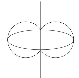
Figure 5.3 Overlay of directional standard deviation and Gaussian ellipsoid (level set of the Gaussian) in . In this example, we overlay a polar plot of the directional standard deviation and a plot of the associated Gaussian ellipsoid (level set). Our plot is in the Principal Order Frame (POF) so that the eigenvectors of the covariance matrix are along the coordinate axes. Notice that along the eigenvectors, the semiaxes of the ellipse are equal to the directional standard deviation. However in directions not along any eigenvectors, the radius of the ellipse is not equal to the directional standard deviation. Credit: Bruce Donald and Anthony Yan.
Finally, we discuss the largest and smallest directional variances. Let be a unit vector in , and let be an arbitrary point set:
From equations (5.24)–(5.26) we see that in general, is a convex sum of the ’s with coefficients . That is, is a weighted average of the ’s. As is well known, the convex sum (convex combination) of points lies within the convex hull of the points. Here, we apply this fact trivially, because our points live in only one dimension, . So our “convex hull” is simply the largest and smallest values of :
PCA is the procedure of computing the eigenvalues and the corresponding eigenvectors , and is used to characterize the directional variances of the data . It is beyond the scope of this book to give a full exposition of PCA. For additional details and applications, we refer the reader to any number of books on statistics, dimensionality reduction, and clustering. It is hoped, though, that this brief introduction will give the reader a solid intuition for PCA. (See the appendix for how to efficiently compute PCA in high dimensions with relatively few data points.)
Residual Dipolar Couplings in Structural Biochemistry
In NMR, we have the interaction of nuclear spins. Intuitively, each spin can be thought of as a magnetic dipole (a tiny magnet) that is spinning like a gyroscope. If there is a very strong external magnetic field, then the dipoles will align themselves with the external field.
In this case, the dipole-dipole interaction of spins can be written as
where and are gyromagnetic ratios of the two spins, is Planck’s constant, is the distance between the two spins, and is the angle between the external field and the internuclear vector (figure 5.4). is a fixed constant equal to . The angle brackets represent an average over time and over the ensemble of proteins in solution, where the scale of the time average is much shorter than can be measured experimentally. For simplicity, we assume here that the nuclei and are covalently bonded, so the distance is not an ensemble average but known from crystal structures.
We now play a series of algebra games, which are the standard manipulations for deriving the Saupe matrix formalism. This is basically the same algebra we used to derive the covariance matrix, where a dot product or a term is expanded as an outer product. To simplify the derivation, let’s normalize and :
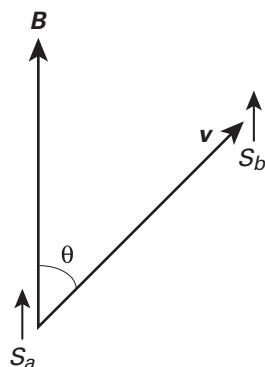
Figure 5.4 Dipole-dipole interaction in a strong external field. If an external magnetic field is very strong, it will align the two spins and ; is the internuclear vector that points from the location of to . is the angle between and . Credit: Bruce Donald and Anthony Yan.
where is the identity matrix.
We now make a physical approximating assumption. Let’s consider our protein to be perfectly rigid. With a rigid protein, we can define a molecular coordinate frame where is constant, and varies because the entire ensemble of proteins are tumbling in solution. Since is constant, we can factor it out:
is known as the Saupe matrix or alignment tensor. is a symmetric, real-valued, and traceless matrix. To show that is traceless, one only needs to show that . Let represent the direction of the magnetic field in the molecular frames of the ensemble of proteins in solution, where . Then,
Consider the trace of each term:
In a homogeneous solution, the distribution of will be spherically uniform since the protein will be tumbling isotropically in all directions. A consequence of this isotropic tumbling is that will become the zero matrix, and the measured RDC effect will be zero. To perform RDC experiments, aligning media are introduced into the solution. The aligning media make the solution anisotropic and cause the proteins to tumble anisotropically. Examples of aligning media include bicelles, phage, and stretched polyacrimide gels. Bicelles are very large flat planar walls of molecules. The wall-like bicelles are packed densely enough that they are roughly parallel, and form a liquid crystal. If the protein is not spherical, then steric collisions with the wall tend to favor some orientations of the protein and disfavor other orientations. As a result, the protein will not tumble isotropically, and the Saupe matrix will not be zero. Other aligning media are believed to work in similar ways, although other aligning effects may be due to charge interactions between surface charges in the media and charges on the protein.
Notice that equations (5.39), (5.42), and (5.43) are similar to a covariance matrix. Because the are not zero-meaned, (5.42) is a pseudo covariance matrix with the identity subtracted off.
While the preceding is the most common formalism presented for the Saupe matrix, we next consider a variation in which we do not assume the protein is perfectly rigid. In fact, we are more interested in the structure and dynamics of the protein than in the Saupe matrix itself. But the same formalism that describes and can be used to characterize the distribution of internuclear bond vectors due to protein flexibility. More precisely, there is an alignment tensor for that has exactly the same form as . Below, we derive this (well-known) formalism.
First, we need a special kind of matrix multiplication, which is essentially the dot product between two matrices.
Definition 5.3 Given two matrices and , which are both , the Frobenius inner product of and is
where and are the component of the respective matrix.
Notice that is commutative and distributive just like the vector dot product. If and are square, this can also be written as where is the trace of a matrix. If is symmetric, then this reduces to .
Now let’s return to equation (5.39), which precedes our assumption that the protein is rigid. Notice we have a term of the form . We have
Furthermore, note that
because .
Using equations (5.50) and (5.51), one can factor equation (5.39) into two parts:
where
At this point, we assume that the overall tumbling of the protein (which determines ) is uncorrelated with the flexing of the protein (which determines in the molecular frame). If two variables are uncorrelated, then the expectation of their product is the product of their expectations:
We define the Saupe matrix .
We define the alignment tensor for to be .
The literature often defines . Different constants may be found in the definition of according to different primary researchers.
If the are identical (i.e., the protein is rigid) in the molecular frame, then mathematically equation (5.61) reduces to equation (5.41).
Both the Saupe matrix and ’s alignment tensor have the same form. For protein flexibility (dynamics), we would like to know the distribution of where the are expressed in the molecular frame. (Because the protein is flexing, a molecular frame may not be well defined; however, it may be reasonably defined.)
It turns out that finding is often an underconstrained problem. However, using a procedure described by Tolman [1], it seems possible to estimate . Tolman’s procedure requires RDCs in five aligning media which is considered to be a high number of media by current experimental standards. Also, Tolman’s problem is underconstrained, so he is required to make some reasonable assumptions, which can be rationalized. Tolman’s procedure can make reasonable (or at least plausible) estimates of .
Once we have , we would like to characterize the distribution in the molecular frame. This, in turn, will help us understand protein flexibility.
Now that we have presented the alignment tensor formalism, and motivated our interest in it, we proceed to the next section where we describe in detail the relationship between alignment tensors and covariance matrices.
RDCs and PCA
In this section we relate RDCs to PCA by showing the connection between the alignment tensor and covariance matrices. To begin, let’s compare the two, side by side.
Let be an arbitrary set of unit vectors.
Our goal is to get as much information about the distribution as possible. In particular, we would like to perform PCA on , or if we can’t, we would like to have as much statistics on as possible.
The two differences between and are that the outer products in are not from zero-meaned vectors, and the final result has the identity subtracted off (The identity can be pulled out of the summation because it is constant, so its average is itself.) As we shall see, subtracting the identity is essentially no problem, but the lack of zero-meaning of the data is a big problem.
First, let us address the subtraction of the identity. It is trivial to see that has the same eigenvectors as , and the eigenvalues of have a simple relationship. This is because, if is an eigenvector of , then multiplication by either or the identity , does not change the direction of :
So if we know and , we can solve for the pseudo covariance matrix . In practice, we know only up to a scale factor, in which case we can solve for up to a scale factor.
Given , we know the pseudo covariance matrix for . What is the relationship between the pseudo covariance matrices and true covariance matrices? As we will show later, the directional variance of a pseudo covariance matrix is an upper bound on the eigenvalues of the true covariance matrix (directional variances of the true covariance matrix). To prove this, we first show that the pseudo covariance matrix of is actually the true covariance matrix of a different point set. Then, we will show that the directional variance of that different point set is always greater than or equal to the directional variance of the original point set . Finally, we will show that if the mean of were known, then we could convert the pseudo covariance matrix into the true covariance matrix for :
We now claim that is the true covariance matrix of . First, we show that is zero-meaned:
Next, we compute the true covariance matrix of and show it is equal to :
Intuitively, we have performed PCA not on the original data , but on “the original data plus its reflection,” namely, PCA on . See figure 5.5 for an example in .
Next, we show that the directional variance of is always greater than or equal to the directional variance of . To do this, we start with zero-meaned data and show that if the data is translated in any direction, the directional standard deviation will remain the same or increase. In fact, the directional variance along the direction of translation will always increase:
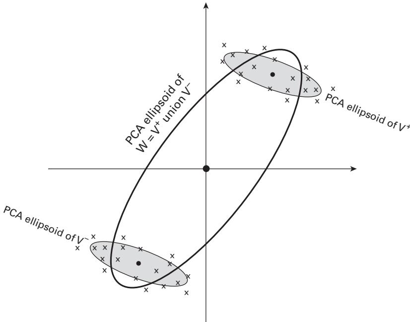
Figure 5.5 PCA of in . The x’s mark the location of data points . The shaded ellipse represents PCA on and is the level set of the associated Gaussian for . The large unshaded ellipse represents PCA on and is the level set of the associated Gaussian for . The means of the three sets , , and are marked by dark filled circles. Credit: Bruce Donald and Anthony Yan.
Let where
By assumption, is zero-meaned:
Let be an arbitrary offset. (5.83)
where
We claim that for any direction , the directional variance of is greater than or equal to the directional variance of . First, let’s consider the covariance matrix of and :
Given the covariance matrices for and , we can now compare their directional variances:
Both and are positive semidefinite, and is also always greater than or equal to zero. So all the terms of equation (5.102) are non-negative. As a result, we can conclude that
Intuitively, the nonzero meaned pseudo covariance matrix always has a larger direction variance than the zero-meaned covariance matrix because the nonzero-meaned case is “stretched apart” by its shadow. (see figure 5.5).
So given (which is equal to ), we have upper bounds on the directional variances of . In the event that we know (which is the mean of ), we can use equation (5.97) to compute the original covariance matrix from the pseudo covariance matrix because . This would allow us to perform PCA on even though we were only given the pseudo covariance matrix.
One might wonder if equations (5.97) and (5.102) can be used to solve for by minimizing . Intuitively, the idea is to find the translation that minimizes the directional variances as much as possible. Unfortunately, this is not the case. The intuition is reasonable, however, we cannot perform all the required steps.
Suppose we are given a pseudo covariance matrix of some point set , which is arbitrary (not zero-meaned). Now we wish to compute the pseudo covariance matrix of , which is the translation of :
We are given only and . Can we compute ? The answer is no:
So we can see that we need to know the average of to solve for . In case that the data is already zero-meaned, then and the above reduces to equation (5.97).
Conclusions and Future Work
Though we don’t know the average from the RDC data, there may be reasonable ways to estimate it based on the area of application. For example, if the protein’s X-ray or NMR structure is known, then the internuclear vectors of the known structure might be reasonable estimates of the average . Given such an estimate, it becomes possible to estimate and perform PCA on .
In some cases, the vectors may be closely clustered on the unit sphere. If their directional variances are much less than unity, then they can be considered to be tightly clustered. In this case, the principle eigenvector of the pseudo covariance matrix may be a reasonable approximation for the average . However, normally in RDC data, the Saupe matrix is nearly zero because the vast majority of proteins are tumbling isotropically in solution. Only a tiny fraction of proteins interact with the aligning media and tumble anisotropically. As a result, we know that the directional variance will be almost the same in all directions, and in fact, the mean will be close to zero. In a sense, we are fortunate that the Saupe matrix subtracts the identity from the pseudo covariance, because if this were not the case, then the eigenvalues of the Saupe matrix would be nearly identical. That, in turn, would make computation of the eigenvectors of the Saupe matrix less numerically stable. If two eigenvalues are equal, their directions must lie in the plane spanned by both of them, but their directions are otherwise unrestricted in that plane. Thus, if the two eigenvalues are nearly equal, their directions are nearly unconstrained in the plane that they span.
Finally, it may be possible to add information or assumptions that result in a lower bound on the directional variances.
Appendix
In this appendix we consider how to compute PCA efficiently when , where is the dimension of our data, and is the number of data points. We are given with . We would like to compute PCA on while not being overwhelmed by .
First, construct a data matrix where the columns are the data vectors :
We can compute the covariance matrix . But, is now , which is huge because . Working with is computationally infeasible. Notice, though, that points in any dimension live in a subspace whose dimension is at most , which is much less than . (For example, three points determine a two-dimensional plane, no matter what dimension the points live in themselves.) So it seems natural to suspect that we can work with a matrix that is rather than .
The matrix is . What is its relationship to ? Notice that both and are symmetric real matrices. So both will have orthogonal eigenvectors. Suppose that we have an eigenvector of :
Then we can multiply both sides by :
So is an eigenvector of with the same eigenvalue .
Similarly, suppose we have an eigenvector of :
So is also an eigenvector of with the same eigenvalue .
As a result, we can solve the eigen-problem for the smaller matrix and then transform the eigenvalues and eigenvectors into solutions of the eigen-problem of the larger matrix . This can save a tremendous amount of computation, and allows PCA to be feasible in practice.
Reference
[1] J. R. Tolman. A novel approach to the retrieval of structural and dynamic information from residual dipolar couplings using several oriented media in biomolecular NMR spectroscopy. Journal American Chemical Society, 124 (2002): 12020–12030.