Chapter 8JIGSAW and NMR
In this chapter, we describe the JIGSAW algorithm [1] for automated NMR peak assignment. A main theme is to see how graph theory is used to develop algorithms in structural biology.
Overview of JIGSAW
JIGSAW is a high-throughput and automated approach for secondary structure determination and resonance assignment from a few, cheap NMR experiments. It applies a graph theoretic framework to represent the atom interactions from the NMR spectra. The contributions of JIGSAW lie in the following parts: First, based on the observation that most protein structures consist of some regular secondary structures, including -helixes, and -sheets, and thus result in certain patterns of NMR-measurable distances, JIGSAW shows that the spectral characteristics of secondary structures can be efficiently identified, and useful for the resonance assignment. Second, JIGSAW implies that a good resonance assignment can be obtained by using the fact that the proton chemical shifts of different amino acid types statistically display distinct patterns in the NMR spectra. Third, JIGSAW can identify -sheets, which are really tertiary structures.
NMR Spectra Used in JIGSAW
JIGSAW exploits the spectra from the following four NMR experiments: NOESY, HSQC, HNH , and TOCSY. The NOESY spectra measure the through-space atom interactions, while the other three spectra measure the through-bond atom interactions. We briefly review these four NMR experiments. Figure 8.1 shows the atom interactions that can be captured by these spectra.
- HSQC is used to capture the through-bond interaction of correlated and atoms. Since every residue has a unique pair on the protein backbone, and thus ideally has distinct frequency signals, the HSQC spectrum serves as the identification of each residue (unassigned), and reference interaction for all other spectra.
- is used to estimate the coupling constant , which is related to the torsion angle of the backbone. Thus, we can infer the secondary structure type from an spectrum.
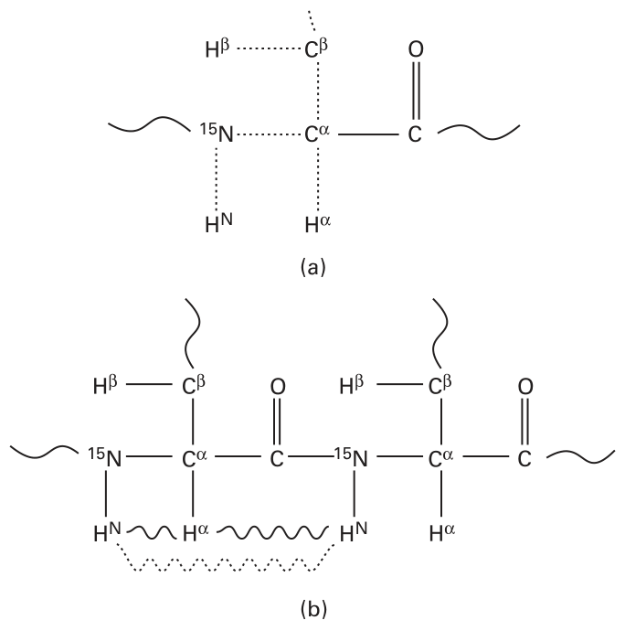
Figure 8.1 NMR interaction graphs showing through-bond and through-space atom interactions in a protein [1]. Atom nomenclature and interactions in a protein. (a) Through-bond interactions shown with dotted lines (HSQC: ; HNH : ; TOCSY: ); (b) through-space interactions in NOESY shown with wavy line ( solid and dashed) [1].
TOCSY The TOCSY spectrum captures the through-bond interactions of protons on a residue’s side-chain. Since the chemical shifts of protons for different amino acids are characteristically different, TOCSY serves as a fingerprint of each amino acid type.
NOESY captures the through-space nuclear Overhauser effect (NOE) between an amide proton and a neighboring in space, which are within a distance less than 6 Å.
Graph Representation of Atom Interactions in NOESY Spectra
Graph Representation
In JIGSAW, the atom interactions from the NOESY spectra are represented by a directed graph , where denotes the set of residues (unassigned, but sharing the same atoms and ), and denotes the set of possible NOESY proton interactions between two residues. Because of the noise in the experimental data, an interaction graph has possible erroneous nodes and edges. There are other characteristics (called “labels”) associated with the nodes and edges in the interaction graph, such as secondary structure type label, match score, and atom distance. For more details, please refer to the definition of “NOESY interaction graph” in Bailey-Kellog et al. [1].
Comment Why should we formulate the proton NOE interactions into directed graphs instead of undirected ones? The reason is that, when two protons are connected to different heavy atoms, the NMR pulse sequence will cause the quantum coherence to transfer along different magnetization pathways.
Graph Constraints for Identifying Secondary Structure
Ideally (if there is no noise), the secondary structures, such as -helix and -sheet, will display certain graph constraints, as shown in figure 8.2. Such graph constraints should correspond to specific subgraphs in the interaction graph.
Secondary Structure Pattern Discovery
The first part of JIGSAW is secondary structure pattern discovery. The input is the NOESY interaction graph, and JIGSAW outputs all the subgraphs that possibly form secondary structures, such as -helix and -sheet. Notice that if the NOESY is perfect, then we can observe some “local” distance patterns (figure 8.3 a) among vertices. Therefore, these local patterns can help us find a secondary structure quickly. Unfortunately, since there are always some false nodes or edges in the interaction graph due to noise in the experimental data, we need to develop algorithms to identify all the subgraphs that are consistent with the secondary structure graph constraints, taking noise into account. JIGSAW applies the following algorithm (figure 8.3 shows the procedure to find -sheet secondary structure from the interaction graph.):
Step 1. Identify instances of fragment patterns.
Step 2. Form sequences of consistent fragments.
Step 3. Form sheets of consistent fragments.
Step 4. Identify the best secondary structure graphs from the set of collected possibilities.
Many fragments can be found in step 3, and they can be inconsistent. Therefore, in step 4, we aim at finding a best consistent fragments graph to be the secondary structure. Of course, there can be many consistent fragments graphs. So, to evaluate a fragment graph , a probability is calculated by multiplying the probability of goodness over all the edges. More precisely, for any edge , let be the weight of (which encodes the differences) in the NOESY interaction graph. Let be the Gaussian prior distribution of width . Then, we define probability of the interaction of to be such that
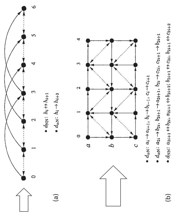
Figure 8.2 Graph constraints [1].
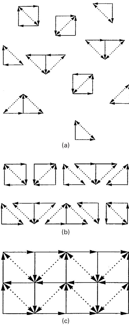
Figure 8.3 Algorithm for identifying -sheets from the interaction graph [1]. JIGSAW algorithm overview: (a) identify graph fragments; (b) merge them sequentially; and (c) collect them into complete secondary graphs. Only correct fragments are shown here. Graphs from experimental data also generate a large number of incorrect fragments, but mutual inconsistencies prevent them from forming either long sequences or large secondary structure graphs.
Then we normalize all the interaction probabilities of all edges generated for the peak of a given edge to define the probability for to be good as such that
where is the set of all edges generated for the peak of .
Finally, the correctness of a graph is defined to be
Then we choose the graph with the largest correctness to be the best secondary structure graph.
Although the interaction graph from experimental NOESY spectra unavoidably includes many false edges, it seems that a self-consistent pattern of continuous false edges is unlikely to occur, based on a simple joint probability model. JIGSAW applies the insight that incorrect edges can be mutually inconsistent, while correct edges can consistently reinforce each other.
Assignment by Alignment of Side-Chain Fingerprints
The BioMagResBank (BMRB) [2] has collected the statistics of observed chemical shifts of the 20 different natural amino acid types, and shown that different amino acid types display distinct fingerprints. The BMRB has been used to predict secondary structure type given chemical shift and amino acid type [2]. The JIGSAW algorithm, on the other hand, predicts amino acid type given chemical shift and secondary structure type. Figure 8.4 shows the mean chemical shifts of the protons for the 20 different amino acid types. JIGSAW applies these distinct “fingerprints” to predict amino acid type, given the chemical shifts from NMR spectra, and secondary structure types discovered. However, since the fingerprint obtained by TOCSY is usually not complete, we need to match the vertex fingerprints (obtained by TOCSY) with the amino acid fingerprints.
The idea of the alignment algorithm is, first, for any fingerprint of residue , denoted by , and for any BMRB amino acid fingerprint , we define the match score by
where is the degree of matching between a subset of of and a subset of , defined as follows:
where is a partial fingerprint matching between and , that is, a bijection between and subsets of .
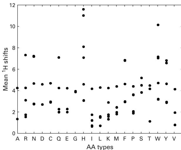
Figure 8.4 The mean proton chemical shifts of the 20 different amino acid types in the BMRB [1]. Cf. figure 3.4.
Then, we define the probability for residue to be amino acid by normalizing the match scores between and all 20 amino acids in as follows:
Now for any sequence of vertices , the beginning position , and the amino acid sequence , we are ready to define the probability of the alignment of and , starting at the th position of :
Finally, we define the alignment between and to be the position that maximizes the probability of alignment starting at any position on , where :
Experimental Results
The following data were used for testing the performance of JIGSAW: the HSQC, HNH , 80ms TOCSY, and 3D -edited NOESY experimental spectra of huGrx, CBF- , and vacGrx proteins. In other tests, synthetic J-coupling constant data were also used in the testing. The results show that JIGSAW is successful in structure discovery and NMR resonance assignment (see figure 8.5 for an example). For more details on the experimental results, please refer to [1].
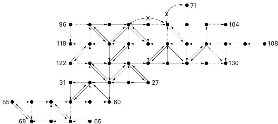
Figure 8.5 -sheets of CBF- computed by JIGSAW. Edges: solid = correct; dotted = false negative; X = false positive [1].
References
[1] C. Bailey-Kellogg, A. Widge, J. J. Kelley III, M. J. Berardi, J. H. Bushweller, and B. R. Donald. The NOESY Jigsaw: Automated protein secondary structure and main-chain assignment from sparse, unassigned NMR data. Journal of Computational Biology 3–4;7 (2000): 537–558.
[2] Eldon L. Ulrich, Hideo Akutsu, Jurgen F. Doreleijers, Yoko Harano; Yannis E. Ioannidis, Jundong Lin, et al. BioMagResBank. Nucleic Acids Research 36 (2007): D402–D408.