Chapter 20Protein Flexibility: Introduction to Inverse Kinematics and Loop Closure Problem
This chapter describes the loop closure problem and inverse kinematics, and their applications in two computational tools for modeling protein backbones: Probik [1] and ChainTweak [2]. We will spend several chapters on the topic of protein flexibility, and computational algorithms to handle it.
Loop Closure Problem and Exact Inverse Kinematics
Protein Backbone Representations
There are two main models to represent a protein backbone: the all-atom Cartesian coordinates-based model and the dihedral angles-based model. Probik applies a Cartesian coordinate-based model, while ChainTweak uses a dihedral angle-based model.
In the Cartesian-based model, an energy minimization step is usually required to compute the correct bond lengths or angles of the protein structure. Due to the efficiency and convergence issues, it is not suitable for larger perturbations of the structure. Although a MD-like approach can be applied to relax this limitation, it incurs an expensive computational cost. Alternatively, the dihedral angle-based model has no restriction on small perturbation size, since no energy minimization step is required. However, a dihedral angle change at one residue position will influence the other positions of all subsequent residues.
Loop Closure Problem
Definition: The -atom Loop Closure Problem Given the fixed positions and orientations of the first and last bonds in an -atom chain, how can one find the possible positions of the internal atoms that satisfy the desired constraints on bond lengths, bond angles, and peptide dihedrals?
It has been shown that the loop closure problem with 6 unknown dihedral angles—that is, 6 degrees of freedom (DOFs)—has at most 16 possible solutions, whereas the number of possible solutions is (generically) infinite for the problem with more than 6 DOFs [3].
Denavit-Hartenberg Local Frames
Consider two bonds, and , as shown in figure 20.1. The Denavit-Hartenberg (DH) local frame on bond is defined as , where are three frame axes, and especially is in the same direction as , and is the origin on bond and closest to bond . To consider the rotational and translational relationship between DH local frames and , we define the following geometric parameters [1]:
: distance along bond from to the closest point to ;
: dihedral angle measured from to about ;
: offset distance from to bond ;
: angle from to .
Let denote the representation of a vector in frame , and let denote the representation of the same vector in frame . Then the relationship between and is formulated as
where , and denotes the homogeneous rotation matrix along the -axis by angle , and denotes the homogeneous translation along the -axis by distance.
Let and denote the DH frames on the anchor and target atoms (respectively) in an -bond chain . The terminology “hand” comes from thinking of the kinematic chain as a robot arm. Let be the representation of a vector with respect to frame , and let be the representation of the same vector in frame . Then we have , where denotes the transformation matrix from frame to .
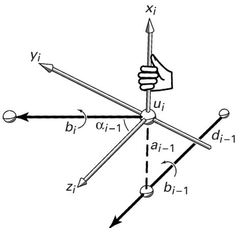
Figure 20.1 Denavit-Hartenberg local frame [1].
Probik
Overview
Probik models the range of possible local motions of the protein backbone by varying the geometric parameters, such as bond angles, lengths, and dihedrals. It computes derivatives of each atom’s position based on an inverse kinematics solver.
Algorithm Description
The following describes the four steps of the Probik algorithm:
- Calculate wiggled loops Compute the geometric representation and parameters of the 6-DOF loop in the inverse kinematics chain, based on the structural information from the PDB file. At the same time, we generate a list of possible values for each variable parameter, based on the actual value, the ideal value, and the standard deviation of this parameter.
- Get exact solutions by using inverse kinematics solver Use the inverse kinematics solver in Manocha and Canny [3] to compute all possible conformations for small variations of one variable parameter at a time.
- Classify families of poses Organize the solution poses and determine the range of allowed motions from the variations of each variable parameter.
- Estimate the derivatives Estimate the derivatives of motion for each atom in the 6-DOF chain. A quadratic polynomial curve, representing a geometric constraint of each atom, is computed to fit the solution poses.
Exploring Control Parameters Based on Principal Component Analysis
Probik uses principal component analysis (PCA) to find a small number of combinations of parameters, acting as “control handles,” that can cover the same space of possible backbone conformations obtained by varying one bond length or angle at a time. The reduction in the number of controls decreases the complexity of backbone manipulation and design.
Probik first generates a large number of perturbed loops by wiggling bond angles and peptide dihedral angles in a normal distribution. Then PCA is applied to compute a low-dimensional approximation of the loop solution space.
ChainTweak
Overview
Given a base conformation, ChainTweak generates a set of backbone conformations within a user-defined neighborhood of this base. Each new conformation has the first and last residues in their same position as in the base, whereas some dihedral angles in between the first and last residues have changed.
ChainTweak uses a sliding window approach to compute the dihedral angles of some atoms within while keeping other atoms fixed. In each window, some perturbations are generated to satisfy the tripeptide loop closure problem.
Algorithm Description
Input A backbone conformation with fixed bond lengths, bond angles, and dihedral angles.
Output A set of conformations whose RMSDs roughly follow a user-defined distribution.
Preprocessing Step Produce a set of conformations by randomly sampling dihedral angles at the end-residues (i.e., dihedral angles near the terminal regions of the chain).
A subroutine based on a sliding window approach, SLIDEWIN, is called iteratively by ChainTweak until a certain large deviation from the starting conformation is achieved. Each iteration of SLIDEWIN moves each residue by around . The output conformation in each iteration is used as the input of the next iteration. Between two iterations, some conformations may be pruned out based on their RMSD from the original conformation and user-defined parameters.
The SLIDEWIN Subroutine Given an input backbone conformation, a window of 3 residues, that is, 9 points, is chosen. Then the residues within the window, that is, with 3 fixed points on both ends, form a 6-DOF loop closure problem, which can be solved by robotics inverse kinematics algorithms, such as that in Manocha and Canny [3]. There are at most 16 possible solutions for each fixed window. A solution within the acceptable regions of the Ramachandran plot is randomly selected as output of this subroutine.
Table 20.1 How Probik and ChainTweak Work
| How They Work | Probik | ChainTweak |
|---|---|---|
| Restrict output to realistic conformations | Must satisfy the 6-DOF loop closure problem | Must satisfy the 6-DOF loop closure problem |
| Loop size | 3 or 4 residues | 3 residues |
| Input backbone size | Unlimited Iterates through all 6-DOF loops in the desired region |
Unlimited “Sliding window” used to iterate through desired region |
| Backbone representation | Cartesian coordinates for atoms and derived joints* | Phi and psi dihedral angles |
| Cover all of the conformational space | Not addressed | “Suggested” to be true, by work on polygonal chains |
Credit: Bruce Donald and John MacMaster.
Table 20.2 What Probik and ChainTweak do
| Probik | ChainTweak |
|---|---|
| “Modeling local protein backbone motion” | “Sampling from the neighborhood of a given base conformation” |
| “Local” = allowed by varying only one peptide dihedral, or bond angle or length within about one standard deviation | “Neighborhood = within 4 Angstroms RMSD of the given base conformation |
| “Provides the biochemist with the range of motions possible for a fragment of the protein backbone” | “Generates a set of backbone conformations” |
Credit: Bruce Donald and John MacMaster. All quotes are from the papers [1, 2].Table 20.3Why the results of Probik and ChainTweak are useful
| Probik | ChainTweak |
|---|---|
| Reduce clashes in X-ray crystallographic refinement | Can improve efficiency of loop modeling programs* |
| Enable backbone movement in protein design | Can generate ensembles to be used to generate decoys* |
| Estimate the derivative of motion for each atom and model each atom’s motion | Being independent of an energy function, can be used in energy function design |
| PCA-based control handles reduce the complexity of protein backbone manipulation* | Can be used in homology modeling to pick the best energy function* |
| PCA-based control handles for loops in alpha-helices are applicable in any alpha-helix* |
Credit: Bruce Donald and John MacMaster.
Comparisons Between Probik and ChainTweak
Tables 20.1, 20.2, 20.3 compare Probik and ChainTweak.
Exercise For each of the “starred” claims (*) in table 20.3, how would you argue these claims are true? For each point, construct a detailed theoretical or empirical demonstration.
References
- [1] K. Noonan, D. O’Brien, and J. Snoeyink. Probik: Protein backbone motion by inverse kinematics. The International Journal of Robotics Research 24;11(2005): 971–982.
- [2] R. Singh, B. Berger. ChainTweak: Sampling from the neighbourhood of a protein conformation. Pacific Symposium on Biocomputing (2005): 54–65.
- [3] D. Manocha and J. Canny. Efficient inverse kinematics of general 6R maipulators. IEEE Transactions on Robotics and Automation 10;5(1994): 648–657.
- [4] Available at http://www4.cs.umanitoba.ca/~jacky/Teaching/Courses/74.795-Humanoid-Robotics/ReadingList/chap3-forward-kinematics.pdf.