Chapter 21Normal Mode Analysis (NMA) and Rigidity Theory
This chapter introduces normal mode analysis [5], and then presents the FIRST algorithm [9] for evaluating the protein flexibility.
Normal Mode Analysis
Introduction
Normal mode analysis (NMA) is a standard technique for studying the dynamics of biological systems. It provides an analytical description of the dynamics in a macromolecular system near a minimum by using a harmonic approximation of the potential. NMA can be applied in the analysis of protein flexibility. It has been shown that over half of the 3,800 Yale database of protein movements can be modeled in a structure using at most two low-frequency normal modes [11].
As shown in figure 21.1, there are two kinds of harmonic approximations of the potential: the local minimum approximation and the effective harmonic (global) approximation. These two approximations correspond to different structural points of view. The effective harmonic approximation overlooks the protein structure (around scale), and thus describes a stable conformation in the overall minimum of potential. In contrast, the local minimum approximation looks closer at the protein structure (around ), and describes a given conformational substate.
The starting point of NMA is finding a particular stable conformation that represents a minimum of the potential energy surface, which can be computed by an energy minimization algorithm. After that, we can construct a harmonic approximation of the potential well around this conformation. A harmonic potential well is defined by
where denotes a -dimensional1 vector describing the stable conformation, denotes the current conformation vector, and denotes a symmetric and positive semidefinite matrix that describes the shape of the potential well. The matrix can be obtained by the second derivative
1 is the total number of atoms.
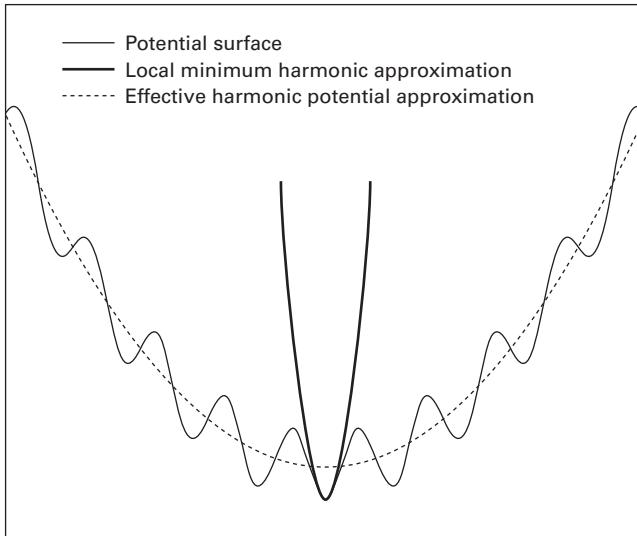
Figure 21.1 Two kinds of harmonic approximations (in one-dimensional view) [8].
of the potential:
where denotes the local minimum.
Figure 21.2 shows the basic idea of normal modes, where denote two coordinates of the system, and denote the normal modes of the harmonic potential well. The motions in the normal mode directions are independent, whereas the motions in the coordinate directions are not. The normal mode vectors can be obtained from the eigenvectors of the matrix :
The associated eigenvalues represents the curve shape of the potential along the normal mode directions.
Based on the independence of the normal modes, we can simplify the harmonic potential function as follows:
where , and , and is a diagonal matrix consisting of the eigenvalues .
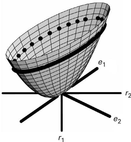
Figure 21.2A two-dimensional harmonic potential well [5].
Different Normal Modes
There are four methods for NMA: vibrational NMA, Brownian NMA, coarse-grained mode, and essential dynamics. Both vibrational NMA and Brownian NMA are derived from a standard all-atom potential by energy minimization, and thus require minimization and Hessian computation. The differences are that vibrational NMA has a short timescale (less than the residence time in a local minimum), and thus is appropriate for studying fast motions, while Brownian NMA has a timescale larger than the residence time in a local minimum, and thus is appropriate for studying slow motions. The coarse-grained mode is used for a given structure, and does not require the expensive minimization and Hessian computation, but instead fits an energy function to the given structure using a spring model. Its timescale is much larger than the residence time in a local minimum, and it is suitable for studying slow, diffusive motions. Essential dynamics is used to find the coordinates that contribute significantly to the fluctuations from a given set of structures that reflect the flexibility of the molecule. It has a timescale much larger than the residence time in a minimum, but cannot capture the fine-level intricacies of the motion. Table 21.1 compares of these four modes.
We recommend the tutorial articles [5, 1] for a more detailed discussion of NMA. A great deal of work has been done on developing and applying NMA methods to analyze biological macromolecular structures, including proteins and ribonucleic acids. For more on these NMA methods and applications see studies listed in the References [2, 3, 4, 6, 7, 10, 12, 15, 16, 17, 18, 19, 20, 21, 22, 23].
Table 21.1 Comparison of normal modes
| Amplitude | Timescale | Starting Structure | Practical | |
|---|---|---|---|---|
| Vibrational | Small | Short | By minimization | N |
| Brownian | Large | Long | By minimization | Y/N |
| Coarse-grained | Large | Long | Given | Y |
| Essential | Large | Long | Given | N |
Protein Flexibility Predictions Using Graph Theory
Overview of FIRST
Given a set of distance constraints, including covalent bonds, hydrogen bonds, and salt bridges, Floppy Inclusion and Rigid Substructure Topography (FIRST) [9] provides the precise mechanical properties of a protein structure. FIRST can compute the rigid regions, and other regions that can move collectively or independently.
Table 21.2 compares FIRST and NMA.
The mathematical basis of the graph theoretic FIRST approach has its roots in Laman’s theorem and a family of algorithms generally known as rigidity percolation, including the “Pebble Game.” We introduce these concepts in the following sections. They are sometimes taught as an allied part of distance geometry (cf. chapters 31, 32, and 36). Most distance geometry algorithms are introduced with the goal of determining a unique or maximum likelihood macromolecular structure. In contrast, in this chapter we discuss rigidity theory from the contrapositive point of view, to calculate flexible regions of a protein. In this light, it is natural to compare and contrast with other methods for modeling protein dynamics, such as NMA. We explore these ideas next.
Rigidity Theory
A protein structure can be formulated into a constraint network, where nodes represent the atoms and edges represent the distance constraints. A constraint is redundant if its breakage does not change the flexibility of the network, otherwise it is considered independent. The following procedure can be used to test whether a constraint is redundant or independent:
- Construct a constraint network representing the structure of the given protein.
- Replace each distance constraint by a spring, and construct a dynamical matrix for the spring network. Then calculate all normal mode frequencies and count the number of zero eigenvalues.
- Add the test constraint to the network, and count the number of zero eigenvalues. If the number of zero eigenvalues remains constant, then the constraint is redundant; otherwise, it is independent.
Table 21.2 Comparison of FIRST and NMA
| All-Atom? | Speed? | Given Starting Pt. | Freq. Spectrum? | Way of Generating New Conformations? | Flexibility or Mobility Index | |
|---|---|---|---|---|---|---|
| FIRST | Y | Y | Y | Low-frequency motion | Y(with ROCK or FRODA) | Y(incorrect for rigid regions flanked by flexible hinges) |
| NMA | Y / N (N for coarse-grained) |
Y (N for VNMA, Brownian, ED) | Y | All frequencies | Y | Y |
This algorithm runs in time, where is the number of atoms in the network. Laman’s theorem is used to calculate the generic rigidity of a 2D framework:
Laman’s Theorem [13, 14] Let be a graph having exactly edges, where is the number of vertices in . Then is generically rigid in if, and only if, for every subgraph of having vertices and edges.
Applying Laman’s theorem directly requires exponential time complexity. However, applying it recursively, as shown in the Pebble Game algorithm [9], takes only time, where is the number of the atoms in the framework.
Notes Laman’s theorem cannot be simply generalized to a 3D framework. So far, it can be generalized only in some special class of 3D frameworks. For more details, please refer to the generic rigidity section in [9].
Pebble Game Analysis
In the 3D Pebble Game algorithm, each node or atom has three pebbles that represent the 3 degrees of freedom of the atom. Each independent edge uses up 1 degree of freedom from one of its incident nodes. We can rearrange pebbles throughout the network while obeying the following pebble covering rule: once an edge has been covered by a pebble, it should be kept covered by one of the pebbles from its incident nodes. Figure 21.3 shows a pebble covering in a network.
The 3D Pebble Game algorithm runs in the following recursive way. Each distance constraint is added at a time, and for each new independent distance constraint, pebbles are rearranged to test whether this constraint is independent. The testing is done by checking whether a pebble can be moved from one of the incident nodes to this new constraint. If a pebble can be collected at both ends, then it is independent; otherwise, it is redundant. This process is repeated until all distance constraints have been placed and tested. From the pebble covering rule, the free pebbles are restricted to certain regions during all rearrangements. The total number of free pebbles on the nodes in a framework represents the number of degrees of freedom associated to this framework. Thus, based on the location and number of free pebbles throughout the framework, we can determine the rigid, overconstrained, or underconstrained regions.
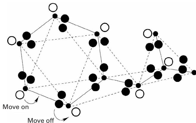
Figure 21.3 A pebble covering. Free pebbles are placed directly on vertices and denote degrees of freedom ( ). Pebbles covering a bond are placed directly on the edges of the graph and represent distance constraints ( ). The pebble covering is not unique, because pebbles can be rearranged according to a few simple rules; see [9]. An example is shown of how an elementary pebble exchange works (two arrows). A free pebble can be moved onto a covered edge (adjacent to a vertex), provided that a corresponding pebble, presently covering the edge and associated with the neighboring vertex, is moved off [9].
References
- [1] I. Bahar and A. J. Rader. Coarse-grained normal mode analysis in structural biology. Current Opinion in Structural Biology 15;5(2005 Oct):586–592.
- [2] B. Brooks and M. Karplus. Harmonic dynamics of proteins: Normal modes and fluctuations in bovine pancreatic trypsin inhibitor. Proceedings of the National Academy of Sciences (U S A) 80;21(1983 Nov):6571–6575.
- [3] B. Brooks and M. Karplus. Normal modes for specific motions of macromolecules: application to the hinge-bending mode of lysozyme. Proceedings of the National Academy of Sciences U S A. 82;15(1985 Aug):4995–4999.
- [4] A. Ghysels, V. Van Speybroeck, E. Pauwels, S. Catak, B. R. Brooks, D. Van Neck, and M. Waroquier. Comparative study of various normal mode analysis techniques based on partial Hessians. Journal of Computational Chemistry 31;5(2010 Apr 15):994–1007.
- [5] K. Hinsen. Normal Mode Theory and Harmonic Potential Approximation, 2000. Available at: http://dirac.cnrs-orleans.fr/~hinsen/.
- [6] K. Hinsen. Analysis of domain motions by approximate normal mode calculations. Proteins 33;3(1998 Nov 15): 417–429.
- [7] K. Hinsen, A. Thomas and M. J. Field. Analysis of domain motions in large proteins. Proteins 34;3(1999 Feb 15): 369–382.
- [8] K. Hinsen. Normal mode analysis: Applications. EMBO practical course on biomolecular simulation. European Molecular Biology Laboratory (EMBL), Meyerhofstr. 1, D-69117 Heidelberg, Germany, 2000. Accessed 2005–2006 at http://dirac.cnrs-orleans.fr/plone/Members/hinsen/courses-and-lecture-notes/embo-course-on-biomolecular-simulations/embo-course-2000/embo\_2000\_normal\_modes\_practical.pdf/view.
[9] D. J. Jacobs, A. J. Rader, L. A. Kuhn, and M. F. Thorpe. Protein flexibility predictions using graph theory. Proteins: Structure, Function, and Genetics 44(2004):150–165.
[10] M. K. Kim, R. L. Jernigan, and G. S. Chirikjian. An elastic network model of HK97 capsid maturation. Journal of Structural Biology 143;2(2003 Aug):107–117.
[11] W. G. Krebs, V. Alexandrov, C. Wilson, N. Echols, H. Yu, and M. Gerstein. Normal mode analysis of macromolecular motions in a database framework: Developing mode concentration as a useful classifying statistic. Proteins: Structure, Function, and Genetics 48;4(2002): 682–695.
[12] O. Kurkcuoglu, Z. Kurkcuoglu, P. Doruker, and R. L. Jernigan. Collective dynamics of the ribosomal tunnel revealed by elastic network modeling. Proteins 75;4(2009 Jun):837–845.
[13] G. Laman. On graphs and rigidity of plane skeletal structures. Journal of Engineering Mathematics 4(1970): 331–340.
[14] Eric W. Weisstein. Laman’s Theorem. From MathWorld—A Wolfram Web Resource. Available at: http://mathworld.wolfram.com/LamansTheorem.html.
[15] G. Li and Q. Cui. A coarse-grained normal mode approach for macromolecules: An efficient implementation and application to Ca(2+)-ATPase. Biophysical Journal 83;5(2002 Nov):2457–2474.
[16] A. D. Schuyler and G. S. Chirikjian. Normal mode analysis of proteins: A comparison of rigid cluster modes with C(alpha) coarse graining. Journal of Molecular Graphics Modeling 22;3(2004 Jan):183–193.
[17] A. D. Schuyler, R. L. Jernigan, P. K. Qasba, B. Ramakrishnan, and G. S. Chirikjian. Iterative cluster-NMA: A tool for generating conformational transitions in proteins. Proteins 74;3(2009 Feb 15):760–776.
[18] F. Tama and Y. H. Sanejouand. Conformational change of proteins arising from normal mode calculations. Protein Engineering 14;1(2001 Jan):1–6.
[19] F. Tama, O. Miyashita, and C. L. Brooks, 3rd. Flexible multi-scale fitting of atomic structures into low-resolution electron density maps with elastic network normal mode analysis. Journal of Molecular Biology 337;4(2004 Apr 2): 985–999.
[20] F. Tama, F. X. Gadea, O. Marques, and Y. H. Sanejouand. Building-block approach for determining low-frequency normal modes of macromolecules. Proteins 41;1(2000 Oct 1):1–7.
[21] A. Van Wynsberghe, G. Li, and Q. Cui. Normal-mode analysis suggests protein flexibility modulation throughout RNA polymerase’s functional cycle. Biochemistry 43;41(2004 Oct 19):13083–13096.
[22] W. Zheng, B. R. Brooks, and D. Thirumalai. Allosteric transitions in the chaperonin GroEL are captured by a dominant normal mode that is most robust to sequence variations. Biophysical Journal 93;7(2007 Oct 1):2289–2299. (Epub June 8, 2007.)
[23] W. Zheng, B. R. Brooks, and D. Thirumalai. Allosteric transitions in biological nanomachines are described by robust normal modes of elastic networks. Current Protein and Peptide Science 10;2(2009 Apr):128–132.