Chapter 23Applications of NMA to Protein-Protein and Ligand-Protein Binding
This chapter describes the applications of NMA to protein-protein interactions [1] and protein-ligand binding [2].
Structure Changes for Protein Binding in the Unbound State
Classical Models for Protein-Protein Interactions
There are three main models for describing the mechanisms of protein interactions: the “lock-and-key” model, the “induced fit” model, and the preexisting equilibrium model, as shown in figure 23.1.
The lock-and-key model emphasizes the importance of shape complementarity between two rigid structures. It cannot be used to explain the conformational changes before and after binding. The induced fit model considers the conformation change due to nonrigid protein interactions. A geometric fit is ensured only after the structural rearrangement of the base protein. In the preexisting equilibrium model, an ensemble of closely related conformations in equilibrium is used to represent the native state of a protein, and for different substrates, there are different suitable conformations to be used for binding. The preexisting equilibrium model can be combined with the induced fit model to explain protein binding.
Gaussian Network Model (GNM)
In a GNM, each residue is represented by a node centered at its atom position. Any two nodes within the distance are connected by a spring of force constant . Thus, we have Gaussian fluctuations for each node and within interresidue distance. The topology of an -node network is represented by a Kirchhoff matrix , that is, for any given , we have
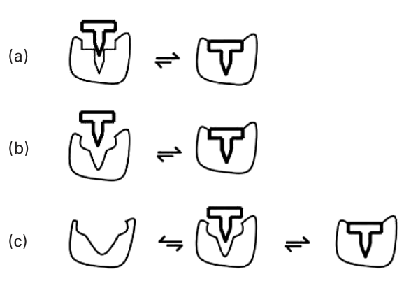
Figure 23.1 Models for protein-protein interactions: (a) Lock-and-key mechanism; (b) induced fit; (c) preexisting equilibrium followed by induced fit [1]. Copyright 2005 National Academy of Science.
The motions along different modes are computed by eigenvalue decomposition , where denotes the orthogonal matrix of eigenvectors, and denotes the diagonal matrix of the eigenvalues , . The eigenvalues represent the frequencies of the nonzero GNM modes, and the th element along the th eigenvector direction represents the fluctuation of residue from its equilibrium position in the th principal axis direction.
The cross-correlation between fluctuations of residues and is
where denotes the inverse of the th element in . The mean-square fluctuation is obtained by replacing by .
The limitation of GNM is that it assumes fluctuations are isotropic, and thus only predicts the motions in their amplitudes, not their directions. On the other hand, the anisotropic network model (ANM), detailed in the next subsection, can provide the directions of collective motions.
Anisotropic Network Model (ANM)
An ANM is a normal mode analysis, where the Hessian matrix is based on a harmonic potential:
where and represent the original and deformed distances between residues and correspondingly. By eigenvalue decomposition of , we have eigenvectors
, where represent the motions of residue in the directions along the th mode.
The ANM modes can be mapped to GNM ones by comparing the squares of fluctuations between the resulting modes in two models.
Receptor Flexibility Representation Through Relevant Normal Modes
Methodology Overview
In Cavasotto et al. [2], a low-frequency normal-mode-based algorithm is presented to generate multiple receptor conformations (MRCs) that incorporate the receptor flexibility in ligand docking and virtual screening. First, we have the following observations:
- The first low-frequency model is not always the best candidate for docking.
- The conformation space grows rapidly with the number of normal modes considered; so does the time complexity.
- Irrelevant modes add noise to energy calculation and minimization.
Based on these observations, the notion of measure of relevance of normal modes on selected regions is used to limit the number of modes for generating MRCs.
The following are the four main steps of the methodology:
- Determine the relevant normal modes that represent binding pocket flexibility.
- Generate a de novo ensemble of MRCs through perturbing the structure along the relevant modes.
- Optimize side-chain conformations by complexing the receptor conformational ensemble with known binders. Minimize the global energy by using a flexible ligand/flexible side-chain approach.
- Screen the generated MRCs by using receptor ensemble docking (RED). Combine the results and search for improvements.
The next sections give the details of these four steps.
Determination of the Relevant Normal Mode
First, a coarse-grained NMA method using atoms is applied. Second, two adjacent regions along the chain are defined, as shown in figure 23.2, where region surrounds the ends of the loop, and region includes the central atoms of the loop. The relevance of mode on the loop is defined by
where
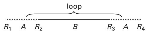
Figure 23.2 Notation in the definition of the measure of relevance [2]. Reprinted with permission. Copyright 2005 American Chemical Society.
Generation of MRCs
Given a set of selected relevant modes, an ensemble of MRCs is generated in the following way:
- Normalize the selected relevant modes.
- Form a linear combination of normalized relevant modes.
- Deform the original structure by displacing all atoms in each residue by the linear combination of relevant modes.
- Generalize an ensemble of conformations by tethering and energy-minimizing the original structure.
- Cluster the structures within the ensemble, and then reduce the number of conformations.
Side-Chain Optimization
The global energy is evaluated and minimized by
- random conformation change according to a predefined probability distribution;
- local energy minimization of differentiable terms followed by global energy reevaluation including nondifferentiable terms; and
- acceptance or rejection on the basis of the Metropolis criterion.
There are three atom layers for side-chain optimization: Zone 1, the ligand plus side-chains within 5.5 Å of the ligand-binding pocket; Zone 2, side-chains within 4.5 Å of Zone 1; Zone 3, the rest of the receptor.
Small-Scale Virtual Screening Using RED
Virtual screening is a strategy using computational analysis to select a subset of compounds appropriate for a given receptor. The following pairs of receptor structures were used for a small-scale virtual screening: 1FMO and receptor A, 1JLU and receptor B, where receptor structures A and B were extracted from complexes A and B. A 1,000-compound library consisting of randomly selected molecules seeded with known cAPK binders was docked and scored to the MRCs using RED. A merging-shrinking procedure was used to sort and merge the screening results, and the best rank for each compound was kept.
References
- [1] D. Tobi and I. Bahar. Structural changes involved in protein binding correlate with intrinsic motions of proteins in the unbound state. PNAS 102;52(2005):18908–18913.
- [2] C. N. Cavasotto, J. A. Kovacs, and R. A. Abagyan. Representing receptor flexibility in ligand docking through relevant normal modes. Journal of the American Chemistry Society 127;26(2005 Jul 6):9632–9640.