Chapter 24Modeling Equilibrium Fluctuations in Proteins
In this lecture, we introduce the fragment ensemble method to capture the mobility of a protein fragment, such as a missing loop, and its extension into the protein ensemble method to characterize the mobility of an entire protein at equilibrium [1, 2].
Missing Loops and Protein Flexibility
Proteins are flexible macromolecules. Under equilibrium conditions, a protein may populate a large ensemble of different structures that could be essential for their biological functions. In particular, loop fragments are sometimes highly flexible even in generally stable proteins, and therefore they cannot always be characterized by X-ray crystallography. In such cases, partially-resolved protein structures are reported with loop fragments missing.
Methods for loop modeling can be broadly classified into two categories. Database methods search for candidate loops that satisfy geometric constraints and constraints on length in homologous proteins available in structural databases, such as Protein Data Bank (PDB) and loop libraries. The limitation of this approach is the loop diversity, which was addressed recently using a divide-and-conquer approach or by assembling long missing loops from small fragments sampled from a loop library. Loops of size up to 15 residues can be modeled by database methods. Ab initio methods may sample from a discretized solution space (e.g., map) and then refine through molecular dynamics simulations, Monte Carlo searches with simulated annealing, genetic algorithms, dynamic programming, bond scaling with relaxation or multicopy searches, or adapt efficient robotics-inspired sampling algorithms to model loops of arbitrary length. Robotics-inspired ab initio methods employ a probabilistic sampling framework: Loop conformations are first sampled ignoring the constraints and later these constraints are enforced through gradient descent, or the satisfaction of constraints is integrated in the sampling process. In the latter case, a loop conformation that satisfies the constraints on its termini is found by solving an inverse kinematics (IK) problem.
Materials and Methods
Fragment Ensemble Method (FEM)
Given an incomplete protein structure and the amino acid sequence of the missing fragment, FEM can generate an ensemble of physical conformations that fit with the given protein structure. The FEM procedure can be described as follows (figure 24.1, plate 26):
Step 0: Obtain initial conformations The unknown fragments (i.e., a missing loop) are initially obtained from a sequence-homologous protein structure from PDB, and the missing atom information is obtained from PSFGEN package. The fragments generally do not fit with the rest of the protein, owing to their nontrivial dependence on the amino acid sequence and the environment provided by the rest of the protein.
Step 1. Backbone geometric exploration An idealized geometry model is used here, and the bond lengths and bond angles are kept fixed to their equilibrium values. The only degrees of freedom (DOFs) employed at this stage are the backbone dihedral angles starting at residue and ending at residue , where the missing fragment is between the residues and . A set of initial conformations for the backbone of the fragment is generated by sampling the values of the DOFs uniformly at random from , and each of these generated fragments was closed by using the cyclic coordinate descent (CCD) algorithm that finds the minimum distance between the residue of the fragment and its target pose in the given protein structure by solving the following IK problem: “Given the positions of the backbone atoms of the stationary anchor , assign values to the DOFs of the kinematic chain modeling the fragment so that the backbone atoms of the mobile anchor assume their target positions in the stationary anchor.” Note that before applying the CCD algorithm, the mobile anchor of the fragment is attached to the corresponding stationary anchor by rigid body transformations. Refer to figure 24.2. In the backbone geometric exploration step, a fragment is said to be collision-free if its energy is below a maximum energy value (i.e., 5,000 kcal/mol).
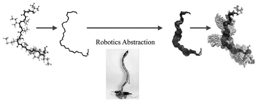
Figure 24.1 (plate 26) Overview of fragment ensemble method (FEM) (1) Backbone geometric exploration: ensemble of backbones that fit the missing loop; (2) side-chain exploration for a fixed backbone: loop in all-atom detail and without steric clash; (3) all-atom energy refinement: energy-minimized ensemble of loops. Credit: Lydia Kavraki.
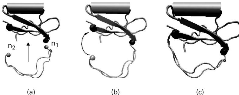
Figure 24.2 (a) The mobile anchors in two different polypeptide chains for the CI2 VAL53-ASP64 loop fragment, drawn in gray, are not attached to the stationary anchors drawn in black. (b) Mobile anchor is attached to its corresponding stationary anchor through rigid body transformations. (c) Rotations of the dihedral bonds of the fragment steer the other mobile anchor toward its target pose in the stationary anchor [1].
Step 2. Side-chain exploration for a fixed backbone In this step, we sample the values of the side-chain dihedrals uniformly at random in the interval until an all-atom fragment conformation is found such that the corresponding protein conformation is collision-free.
Step 3. Energetic refinement of a modeled fragment The closure-constrained backbone refinement and the closure-constrained conjugate gradient descent strategies are performed in this step to refine each completed protein conformation generated from the last step. The first strategy is to minimize the energy of a completed protein conformation while keeping the fragment anchored and modifying the dihedrals during minimization, and the latter method relaxes the idealized geometry model and allows more mobility of the fragment’s atoms for stable interactions with the rest of the protein. Since both of the aforementioned methods can be trapped in local minima, an interleaving minimization procedure used the two preceding methods in interleaving mode in the hope of discovering a better energy minimum (which can still be a local minimum, if we are unlucky).
FEM yields many all-atom closed fragment conformations of low energy, and the work [1] indicates that the fragment conformations can be generated independently from one another and their computations are easily distributed. Also, it is possible to employ a Boltzmann probability-based statistical mechanics model to weight the probability of a local fluctuation.
Protein Ensemble Method (PEM)
PEM, which employs FEM as a component to capture equilibrium fluctuations over an entire protein, has the following three steps.
Step 1. Define consecutive overlapping fragments The polypeptide chain of the protein is divided into a set of consecutive fragments with significant overlap to characterize the flexibility of the entire protein. In Shehu et al. [1], the fragment size (or window size) is chosen to be 30 residues long and the overlap between two consecutive fragments is 25 residues.
Step 2. Obtain fragment ensembles For each fragment , an ensemble of physical fragment conformations are obtained using FEM.
Step 3. Combine fragment ensembles The fluctuations of the overlapping fragments are combined to obtain equilibrium fluctuations of the entire chain. Any measurable quantity for residue can be obtained as a weighted average of the values measured for the residue over all the overlapping fragments in which residue is present. For example, if the window size and the overlap are set to be 30 and 25, respectively, the residue 19 is then contained in fragments [1, 30], [5, 35], [10, 40], and [15, 35]. Here the square brackets denote fragments, e.g., [1, 30] is residues [1 – 30]. Therefore, any measurable quantity , for can be obtained independently over these four fragment ensembles , , , and . Finally, the average value , is defined by averaging over all the different fragment ensembles embracing residue , as
in which is the normalization factor and is the weight function used to downplay the finite-size effects introduced by the finite length of each fragment. Furthermore, the contribution of the terminal residues of each fragment and a few neighboring residues to the total average needs to be either discarded or strongly reduced, because they are attached to the reference protein structure through the CCD algorithm, and hence are artificially restricted.
Measuring Robustness to Different Approximations Following is a list of approximations to measure their effects on the equilibrium mobility captured:
- The order of update of the DOFs in the CCD algorithm. (N terminus to C terminus or random order).
- Inaccuracy of the force field employed: CHARMM versus AMBER.
- Finite-size effects because of the definition of the fragments and inherent to the CCD algorithm.
- Energy minimization of obtained conformations (can be trapped in a local minimum).
- Statistical weighting scheme and the weight functions used.
The errors from these approximations compared to the error bars for ensemble averages of NMR data such as residual dipolar couplings and order parameters indicate that these approximations do not significantly affect the equilibrium mobility of the proteins employed (refer to figure 24.5).
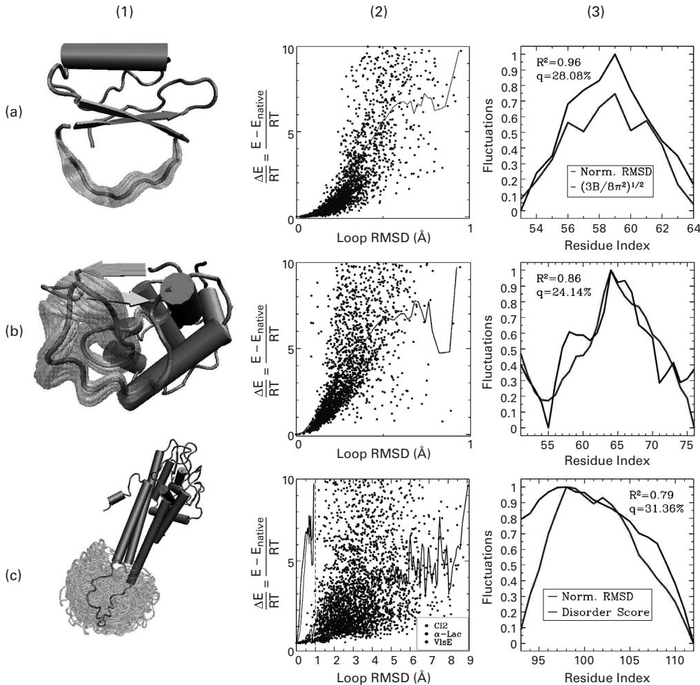
Figure 24.3 (plate 27) (a1, b1, c1) 5,000 transparent loop conformations versus opaque reference structure (equilibrated native structure for CI2 and -Lac and lowest energy structure for VIsE). (a2, b2, c2) Energy landscapes associated with generated ensembles are shown by plotting the energetic difference versus the RMSD of each conformation relative to a reference structure. Energy landscapes are shown only for conformations with energy less than 10 RT units away from the reference structure. An average energy profile is computed by distributing conformations in bins every 0.001 Å away from the reference structure and measuring the energy of each bin as an average over its conformations. Average energy profiles obtained for CI2 and -Lac are very steep compared to the flat average energy profile of VIsE. (a3, b3, c3) Obtained fluctuations versus B factor-derived fluctuations for the CI2 loop, fluctuations in the literature for the -Lac loop, and disorder scores for the VIsE loop [1].
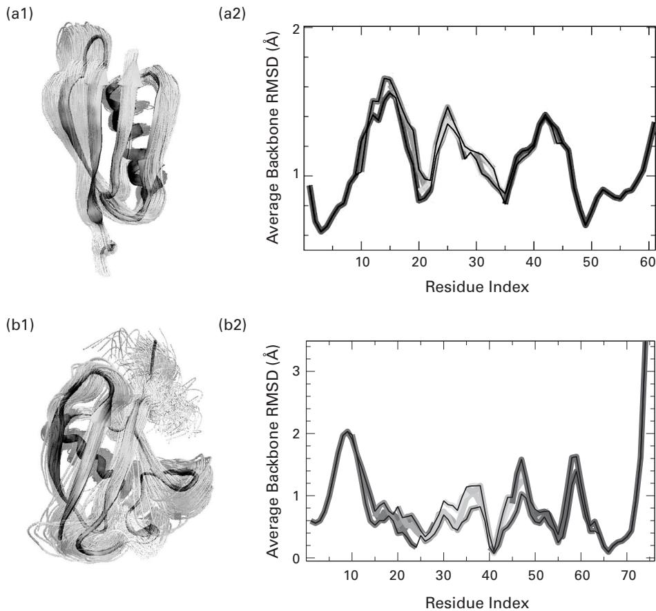
Figure 24.4 (plate 28) (a1 and b1) Computed native ensembles for protein G and ubiquitin, respectively. (a2 and b2) Average RMSD per residue obtained by combining the local fluctuations of all the different regions. Results for different regions are shown in different colors, from red to blue as a window of 30 residues slides from the N- to the C-terminus of the protein. The black lines mark the highest and lowest RMSD values recorded from all the different windows including each given residue, and provide an estimate for the uncertainty of the procedure. Two consecutive 30-residue windows have an overlap of 25 residues. The results corresponding to the first and last 5 residues of each fragment are discarded since they are biased by the finite size of the window [1].
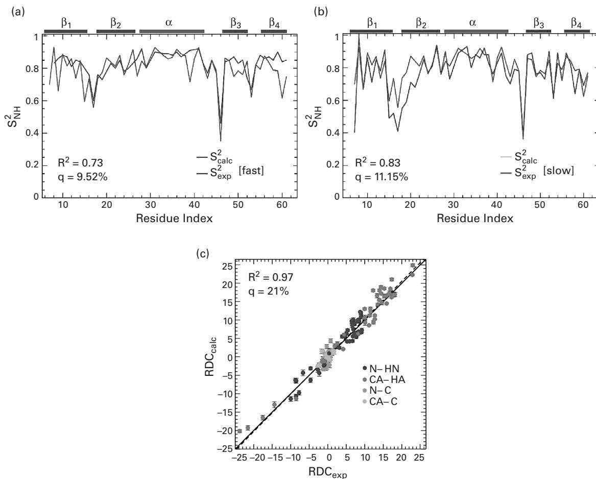
Figure 24.5 (plate 29) Comparison of NMR relaxation data measured versus the generated ensemble for protein G. (a) Comparison of backbone (amide) order parameters calculated over the ensemble ( ) with fast ( ) data obtained from NMR relaxation measurements ( ). (b) Comparison of backbone (amide) order parameters measured over the ensemble ( ) with slow ( ) data obtained from NMR relaxation measurements ( ). (c) Comparison of residual dipolar coupling (RDC) parameters as obtained in the ensemble ( , on the y-axis), and from NMR relaxation measurements ( , on the x-axis). Results for different bond types are shown in different colors. (a–c) The dashed black line indicates the linear least-squares regression fit on the two sets of data, while the continuous line represents the identity diagonal [1].
Therefore, it is reasonable to combine the results obtained in different fragments to generate global fluctuations over an entire protein.
Results
To validate the accuracy of FEM, as shown in figure 24.3 (plate 27), the work [1] reproduces some native loops in stable proteins, such as CI2 (PDB ID: 1COA, 12-residue loop between VAL53 and ASP64), and -Lac (PDB ID: 1HML, the 26-residue loop between LYS51 and THR76).
Figure 24.4 presents the results of the application of PEM to characterize the equilibrium ensemble of two proteins: streptococcal protein G (PDB ID: 1IGD) and human ubiquitin (PDB ID: 1UBQ). Figures 24.4 (a1) and (b1) qualitatively show the structural variability of the generated structures for protein G and ubiquitin. The consistency of fluctuations measured over ensembles of neighboring overlapping fragments can be seen in figure 24.4 (a2) and (b2), where the average RMSD of each residue measured over ensembles of the fragments that encompass that residue is plotted. See plate 28.
Order parameters—experimentally available data for protein G—are derived from NMR relaxation experiments and capture the fast dynamics of this protein in the picosecond to nanosecond timescale, which we refer to as fast . Figure 24.5a shows the agreement between the ensemble-calculated backbone (amide) and the fast data of protein G. The agreement is better for -helix and the - and -helix loops (residues 22–48), indicating that most of the mobility captured by the ensemble for these residues happens on the picosecond to nanosecond timescale. Figure 24.5b shows a better agreement between the data measured over the ensemble and the slow data reported in literature. In figure 24.5c, it is shown that the RDCs measured over the ensemble and those experimentally measured in bicelle medium agree with a Pearson correlation of 97% and q-factor of 21%.
Exercise In order to compare RDCs from the computationally-predicted ensemble versus experimental RDCs, how should the alignment tensor(s) be computed? And how should the back-calculated RDCs be weighted in calculating the ensemble average?
References
- [1] A. Shehu, C. Clementi, and L. E. Kavraki. Modeling protein conformational ensembles: from missing loops to equilibrium fluctuations. Proteins: Structure, Function, and Bioinformatics 65;1(2006 Oct 1):164–179.
- [2] Available at: http://www.cs.rice.edu/CS/Robotics/bioinformatics/EquilibriumFluctuations.html.