Chapter 25Generalized Belief Propagation, Free Energy Approximations, and Protein Design
In this chapter we introduce graphical models and belief propagation algorithms. Then we discuss two applications. First, we describe a generalized belief propagation algorithm for approximating the free energy of a protein structure. Second, we describe how belief propagation algorithms can be useful in protein design.
Graphical models are a powerful, and relatively new algorithmic framework, which shows significant promise for structural biology.
Free Energy
A general definition for the free energy of a system is “the amount of energy which can be converted into work.” Although there are several types of free energy, the most widely used is the Gibbs free energy, which can be defined as the amount of thermodynamic energy that can be converted into work at constant temperature and pressure. Formally, we write
where = Gibbs free energy, = enthalpy (the heat content of the system), = entropy (a measure of the degree of randomness of the system), = internal energy, = absolute temperature, = pressure, and = volume.
The change in the Gibbs free energy of a system is , and since the change in volume is small for nearly all biochemical reactions, we can write .
Free energy functions have been successfully used in protein structure prediction, fold recognition, homology modeling, and protein design; for example, see chapters 11 and 12. However, most free energy functions only model the internal energy using inter-and intramolecular interactions terms (van der Waals, electrostatic, solvent, etc.) [11, 13, 8, 2]. The entropy is usually ignored because it is harder to compute, since it involves summing over an exponential number of terms. Another approach is to compute the free energy using statistical potentials derived from known protein structures (e.g., from PDB). Such methods have the advantage that the derived potentials encode both the entropy and the internal energy . But there are several disadvantages, the most important being the fact that the observed interactions are usually not independent [14]. Kamisetty et al. [15] use a generalized belief propagation algorithm to compute an approximation of the free energy function that includes the entropy term.
Graphical Models
Graphical models are graphs that represent the dependencies among discrete random variables. The variables are usually represented as nodes in the graph and the dependencies as edges. Examples of graphical models include Bayesian networks (figure 25.1a), Markov random fields (figure 25.1b), and factor graphs (figure 25.1c). We use capital letters for the random variables () and small letters for the discrete values that the random variables can take ().
Let be the joint probability of all the variables in the model. The marginal probability of each variable can be written as
Computing these marginal probabilities is usually computationally expensive because it involves a sum over an exponential number of terms. Belief propagation algorithms try to overcome this problem by approximating the marginals with the beliefs .
Bayesian Networks
In a Bayesian network (BN), the dependencies (conditional probabilities) are represented by arrows. Each variable is independent of all the nondescendants, given its parent. For example, for the BN in figure 25.1a we have . The joint probability can be written as
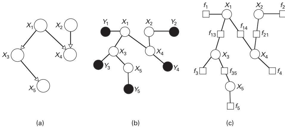
Figure 25.1 (a) Bayesian network. (b) Pairwise Markov random field. (c) Factor graph.
Pairwise Markov Random Fields
A Markov random field (MRF) contains two types of random variables: hidden () and observed (). The dependencies among variables are represented using compatibility functions (also known as potentials): the local evidence for (sometimes written simply ), and the compatibility between and . In this case we call the MRF “pairwise” because the potential functions are defined pairwise.
The joint probability for a pairwise MRF can be written as
where is a normalization constant, also called the partition function.
Factor Graphs
In a factor graph (FG) the interactions between variables are represented by the factor nodes (the square nodes in figure 25.1c), and the joint probability can be written as a product of all the factors: . For example, for the FG in figure 25.1c we have
It is important to notice that all three graphical models described here (BNs, pairwise MRFs, and FGs) are equivalent in terms of the systems they can model [20]. In particular, the equivalence of pairwise MRFs and FGs can be illustrated by the equivalence between the compatibility functions and the factors:
Belief Propagation (BP)
Belief propagation is a method for approximating the marginal probabilities in a graphical model, in a time linear in the number of variables (nodes). BP is precisely mathematically equivalent for pairwise MRFs, BNs, and FGs. However, it is easier to explain on a pairwise MRF.
Let be the hidden variables. We define a message from a node to a node as an array containing information about what state node should be in. For example, if can take the values 1, 2, or 3, then the message can be interpreted as follows: node is telling node that it should be in state 1 with probability 0.7, in state 2 with probability 0.1, and in state 3 with probability 0.2.
BP is an iterative algorithm. It starts with randomly initialized messages and then it applies the message update rule below until the messages converge:
where and are the potential functions and is the set of all neighbors of node . After convergence, the beliefs (the approximate marginals) can be computed as
When the MRF has no cycles, the computed beliefs are exact! Even when the MRF has cycles, the BP algorithm is still well-defined and empirically it often gives good approximate answers.
The Connection between Belief Propagation and Free Energy
We can write the Gibbs free energy of a system as , where the entropy is ( iterates over all possible states of the system).
For a graphical model, if is an instantiation of all the random variables (or equivalently, the state of the model), we can write the joint probability as using Boltzmann’s law as . is the partition function. Notice that we consider and we ignore Boltzmann’s constant (which affects only the scale of the units).
Using BP, we approximate the joint with the belief . To see how close these two distributions are, we can use the Kullback-Leibler distance (cf. chapter 13):
Notice that the second equality was obtained by substituting as defined using Boltzmann’s law.
Two important properties of the KL distance are that it is never negative, and it becomes zero if and only if the two probability distributions are exactly the same. In this case, we have
In other words, when the beliefs are exact, the approximate Gibbs free energy achieves its minimal value – , also called the “Helmholtz free energy” [21].
Generalized Belief Propagation (GBP)
Computing the Gibbs free energy involves summing over an exponential number of terms, which is usually computationally intractable. Instead, several approximations of the free energy have been developed:
- Mean-field approximations use only one-node beliefs;
- Bethe approximations [22] use one-node and two-node beliefs; and
- Region-based approximations are based on the following idea: Break up the graph into a set of regions, compute the free energy over each region and then approximate the total free energy by the sum of the free energies over the regions.
Region-based approximations can be computed using generalized belief propagation (GBP), a message-passing algorithm similar to BP. GBP uses messages between regions of nodes instead of messages between nodes. The regions that exchange messages can be visualized as region graphs [21].
Different choices of region graphs give different GBP algorithms. There is usually a tradeoff between complexity and accuracy. However, how to optimally choose the regions is still an open research question. One heuristic I advise is: try to include at least the shortest cycles inside regions.
Similar to BP, GBP is guaranteed the give the optimal solution when the region graph has no cycles, but it also works very well on many graphs that contain cycles. In [21], Yedidia et al. try to understand why GBP works on graphs with cycles, and they offer some guidelines for constructing region graphs for which some theoretical guarantees can be offered.
An Application of GBP: Estimating the Free Energy of Protein Structures
Kamisetty et al. [15] use GBP to estimate the free energy of all-atom protein structures. They model the structure of a protein as a probability distribution using a pairwise MRF:
- The observed variables are the backbone atom positions (continuous).
- The hidden variables are the side-chain atom positions represented using rotamers (discrete).
- Two variables (atoms) share an edge (interact) if they are closer than a threshold distance, set to 8 Å.
- The potential functions are defined as
where is the energy of interaction between rotamer state of residue and rotamer state of residue . See figure 25.2 (plate 30).
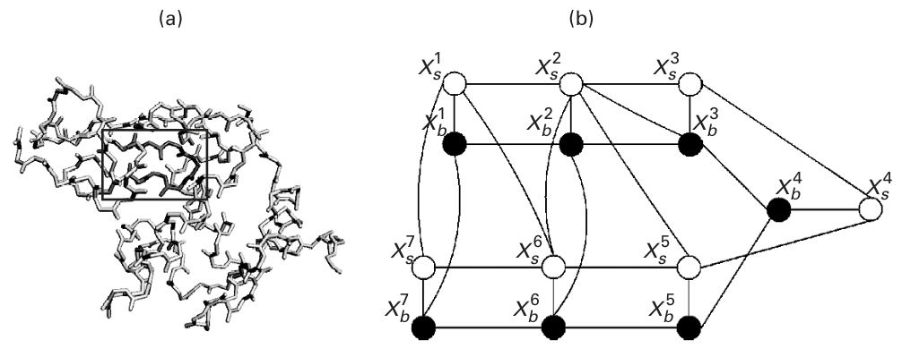
Figure 25.2 (plate 30) (a) Structure of lysozyme (PDB id: 2lyz) with a few residues highlighted. (b) Part of the random field induced by the highlighted residues: ’s are the hidden variables representing the rotameric state, the visible variables are the backbone atoms in conformations [15]. The publisher for this copyrighted material is Mary Ann Liebert, Inc. publishers.
After building the pairwise MRF, Kamisetty et al. transform the MRF into the equivalent factor graph. Then, they split the factor graph into regions: big regions containing two or three variables and small regions containing just one variable (see the examples in figure 25.3). The basic idea behind the choice of regions is: place residues that are closely coupled together in the same big region. This idea was borrowed from Aji and McEliece [1], and it provides a balance between the accuracy of the approximation and the complexity of the model.
The region graph is then built by drawing an edge from each big region to all the small regions that contain a strict subset of the big region’s nodes. Finally, a GBP algorithm called “the two-way algorithm” [21] is applied on the resulting region graph.
Results and Discussion
Kamisetty et al. use the entropy component of their free energy estimate to distinguish between native protein structures and decoys (structures with similar internal energy to that of the native structure, but otherwise incorrect). They find that when the structures are ranked in decreasing order of their entropy, the native structure is ranked the highest in 87.5% of the datasets that contain decoys with backbones similar to the backbone of the native structure, and 84% of the datasets that include dissimilar backbones.
The authors also compute estimates of the on mutation and their results correlate reasonably well with the experimental values (with correlation coefficients varying from 0.63 to 0.7, and -values between and 0.0063).
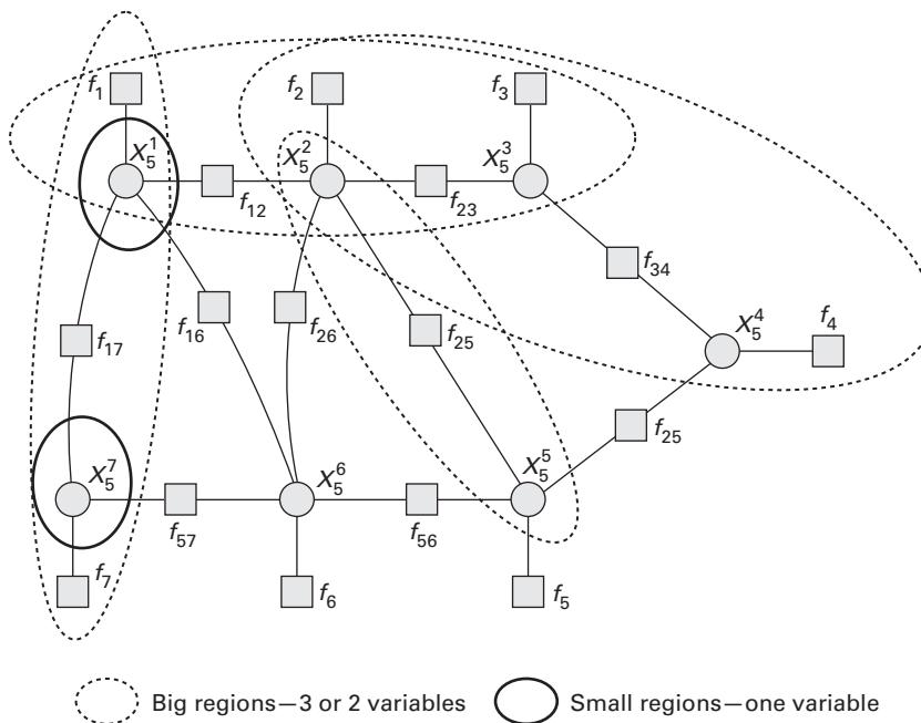
Figure 25.3 The factor graph with regions.
We have learned about a method for estimating side-chain conformational entropy using belief propagation. The algorithm (chapter 12) also models free energies from conformational ensembles. While belief propagation techniques are usually probabilistic or stochastic, the algorithm is deterministic and operates by computing provably good approximations to the partition functions [13, 8, 2].
Up to now, this chapter has considered belief propagation for ensemble properties (such as conformational entropy). Belief propagation algorithms are also useful in the search for the global minimum energy conformation (GMEC) of protein side-chains, which is an important computational challenge in protein structure prediction and design (see chapters 11–12). We discuss belief propagation algorithms for protein design in the next section.
Application: Graphical Models for Protein Design
In section 25.6 we introduced a method based on generalized belief propagation to estimate the free energy of a protein structure. Free energy is composed of both an enthalpic term and an entropic term.
Protein design frequently involves searching for a sequence of amino acids that will fold to a target structure or will perform a desired function (chapters 11, 12). Ideally, we would search for the sequence with the lowest free energy, accounting for both enthalpy and entropy since entropy has been shown to be important when scoring mutants of proteins [13, 2, 8].
The entropic component, however, is commonly ignored in protein designs for several reasons. First, it is often assumed that entropy plays a smaller role in the stability and function of a protein [10]. Second, entropy calculations must account for an exponential number of states (conformations) for each sequence. Finally, in most techniques for entropy calculations, like the method introduced in section 25.6 and the algorithm (chapter 12), entropy must be computed at least partially for each sequence, and therefore an exponential number of sequences must be considered.
For the remainder of this chapter, we consider belief propagation as an aid to protein design in which the enthalpy is modeled but the entropic and ensemble properties of section 25.6 and chapter 12 are explicitly ignored. This corresponds to the “classical” inverse folding problem introduced in chapter 11. Recall that this restricted protein design paradigm involves an input model, a protein design algorithm that performs a search over a combinatorially large sequence space, and the output of one or more candidate sequences (chapter 11). Input models are chosen with computational feasibility in mind. A common input model used in protein design assumes a fixed backbone for the protein, a discrete number of conformations possible for each side-chain, and a pairwise additive energy function. This simple model is convenient because it reduces the continuous conformation space to a discrete space with a finite number of conformations. The search over the discrete space, however, remains intractable and the problem of assigning discrete rotamers has been shown to be NP-hard.
Provable algorithms like DEE/A* [12] can solve many instances of the basic problem of finding the global minimum energy conformation. Nevertheless, there are instances of the problem where the state of the art in provable algorithms might not be able to find a solution in a reasonable amount of time.
As we explained at the beginning of this chapter, graphical models are a graph representation of conditional independence between random variables, while Belief Propagation (as presented in section 25.3) is a method to compute the probability distribution of each of the random variables by passing messages between variables. Messages encode the belief one neighbor has about another and are propagated during sequential iterations throughout the graph. In protein design, the random variables are residues that can be in a discrete number of states (i.e., rotamers). The neighbors of each random variable in the graphical model are the residues that are close enough to interact.
We will present three variations of the protein design problem for which the use of Belief Propagation as defined in section 25.3, is useful: search for the global minimum energy conformation, enumeration of the best low-energy sequences, and probabilistic protein design. We build on earlier chapters discussing the protein design problem, energy functions, dead-end elimination (DEE), rotamers, and algorithms for NP-hard problems.
Protein Design Problem
We first define the protein design problem as in chapter 11 and Fromer and Yanover [5], where a fixed backbone and a discrete, finite number of rotamers is assumed. Rotamers of different amino acids are treated uniformly, and we search for a single assignment of rotamers at all of the redesign positions that will have the lowest energy: the global minimum energy conformation (GMEC). We are interested in the amino acid sequence of the GMEC (i.e., the amino acid type of each rotamer). In contrast to chapter 12, under this definition of the protein design problem, the terms “conformation” and “rotamer assignment” are equivalent, since rotamers are always in a single, rigid state.
Let denote an assignment of rotamers in positions. Let be the self-energy of rotamer and the pairwise energy between rotamers and . We define the energy for the rotamer assignment , as
Let be an amino acid assignment; let be the amino acid type of the rotamer assigned at position , and the amino acid assignment for rotamer assignment . We define the minimum energy of a sequence as
and the problem of searching for the minimum energy sequence as
Protein Design as an Inference Problem We now recast the protein design problem as an inference problem by using Boltzmann-weighted terms for all energy interactions [5]. Let
where is the system temperature. We define the probability of each rotamer assignment,
where is the normalization factor (i.e., the partition function, which guarantees that the sum of the probabilities over all states equals 1). Finally, analogous to equation (25.4), we define the problem of finding the sequence that contains the rotamer assignment of highest probability:
Graphical Models and Belief Propagation for Protein Design
Long-range interactions in protein design models tend to be weak. The choice of rotamers in two residues that are far away from each other will most likely have little direct influence on each other, but indirect influence is more likely (e.g., a “domino” effect). We take advantage of weak long-range interactions to build a graphical model where an edge exists between a pair of nodes if they have a significant interaction.
In protein design, we must find conformations that have globally low energy. Any algorithm that searches for low-energy conformations must account for the effect of local choices on the overall global energy. In belief propagation, a random variable receives a message from each of its neighbors, telling it what they think the probability of each of its rotamers should be. The message encodes both local information (i.e., the intrarotamer energy at each position and the energy interactions with each neighbor), and global information, which is encoded (indirectly) through the relayed effect of messages from neighbors of neighbors. On each iteration, only messages from immediately adjacent neighbors are incorporated into the probabilistic score of each rotamer at a position. But on successive iterations, the belief is propagated through the entire graph.
Formally [5], a rotamer receives a message from each of its neighbors containing information about the “belief” that each neighbor has about the probability of residue position being in state :
Note that is a vector with dimension equal to the number of possible rotamers at . Initially, all messages are set to 1 (or a normalization of it). Messages are updated on all nodes until convergence or a fixed maximum number of iterations. Within each iteration, nodes can be selected sequentially for updates. If the graphical model is a tree, the belief propagation algorithm will converge. In “loopy” belief propagation (i.e., graphs with loops) there is no guarantee for convergence.
Each rotamer is a member of an exponential number of rotamer assignments. The protein design problem (eq. 25.4) consists of finding the rotamer assignment of lowest energy. In equation (25.9) we take the maximum over all incoming messages to , and the resulting message value is the function of only one of the rotamers in . This type of belief propagation is called max-product belief propagation. Contrast this with the definition in section 25.3, where all the incoming messages are added, which is called sum-product. For each rotamer, we will approximate the marginal probability of the lowest-energy (and highest-probability) rotamer assignment that rotamer is part of, as a function of incoming messages and the internal energy of . This is referred to as max-marginal probability ():
If belief propagation converges, then approximates the exact max-marginal of , denoted , which represents the maximum probability (eq. 25.7) over all rotamer assignments that contain :
Finally, we select a rotamer assignment such that the max-marginal probability of each rotamer in the assignment is maximized over the possible values of :
where is the set of rotamers allowed in position . If we can converge to exact max-marginals (i.e., if , for all ), then .
Multiple Low-Energy Sequences Through BP
The protein design problem as defined in equation (25.4) searches for a single sequence that contains the GMEC. In practice it might be desirable to have several low-energy sequences for the following reasons. Some parts of energy functions for computational protein design are developed by fitting to experimental data, which might lead to overfitting. Assumptions about proteins in the model, like discrete rotameric states and a fixed backbone, might produce inaccurate results. Provable algorithms that produce combinatorially precise results are usually slower than inexact, sampling methods, but the sequences enumerated by inexact algorithms might not be good. Finally, predicted low-energy structures might be too stable, not fold to the target structure, or lack binding affinity to a substrate. By generating a large set of low-energy sequences, we can increase the likelihood that one of them will fold to the target structure and have the desired properties.
The DEE algorithm is efficient in pruning conformations that are provably higher in energy than other conformations. If we wish to avoid pruning of other low-energy sequences, we must choose a threshold value for an energy window so that no conformations within of the lowest-energy conformation are pruned.1 Provable algorithms generally are not designed to enumerate more than the single lowest-energy sequence (i.e., the GMEC) since they make no distinction between whether two rotamer assignments belong to the same sequence or to different sequences. In DEE/A*, for example, in the worst case, a low-energy sequence with an exponential number of low-energy rotamer assignments might have to be enumerated fully before the next lowest energy sequence can be enumerated.
Fromer and Yanover [5] propose the tBMMF (type-specific Best Max-Marginal First) algorithm, that provably enumerates low-energy sequences in order of increasing energy if the belief
1 Techniques like MinBounds [7] enable more efficient pruning of rotamers with energies above , when is large, but might not be as efficient as DEE with . Therefore, problems that might be tractable when searching for a single minimum energy structure, might be slow to solve when multiple low-energy sequences are desired.
propagation algorithm converges to exact max-marginals; unfortunately, exact max-marginals are only guaranteed to converge on tree graphs. Type-dependent dead end elimination (tdDEE) [19] is used to reduce the search space, while guaranteeing that no sequences will be pruned. At least one rotamer of every allowed amino acid at each position is not pruned by tdDEE.
Intuitively, the tBMMF algorithm works as follows. The algorithm first computes the max-marginals as in section 25.7.2 and enumerates the lowest-energy sequence. The max-marginal for each rotamer (eq. 25.10) is an approximation to the probability (eq. 25.7) of the lowest-energy rotamer assignment in which is present. If (eq. 25.12) is the sequence of the rotamer assignment of lowest-energy, the next lowest energy sequence must differ by at least one amino acid from . Let be the rotamer with the lowest max-marginal such that . Then we know that the probability of the next lowest energy sequence is that of (the best max-marginal), and that is part of the next lowest energy rotamer assignment.
We cannot, however, know which other rotamers belong to the next lowest-energy rotamer assignment. The tBMMF algorithm therefore partitions the search space into two subspaces: one that contains the amino acid as the lone amino acid at position and another subspace that doesn’t contain amino acid , at position . BP is then performed on both subspaces; in the subspace that contains , we should find the second lowest-energy sequence, and we compute the max-marginal of the next lowest-energy sequence in that subspace. In the space constrained to all the amino acids except , should again be the lowest-energy sequence, but a different amino acid should be the next best max-marginal since is not present in this subspace. We then choose between the two max-marginals and repeat the process. Using the toy system in figure 25.4, figure 25.5 shows an example of this process. For a detailed description of the algorithm and proof of its correctness under exact max-marginals, refer to Fromer and Yanover [5].
Graphical Models for Probabilistic Protein Design
Phage display is an experimental method where a large number of random peptide sequences ( – ) can be screened for binding to another protein or ligand. Even with libraries this huge, however, we still can’t evaluate the exponential number of peptide sequences that arise as we increase the number of design positions and choice of amino acids at each position. With a choice of 20 amino acids per position, even a small peptide with 10 amino acids would have sequences, a thousand times more than what we can handle with current phage display techniques. The distribution of amino acids at each redesign position, however, can be biased toward amino acids that will yield low-energy conformations of the target backbone.
In probabilistic protein design, a probability distribution is assigned to each design position, and correspondingly, each amino acid is assigned a probability. Fromer and Yanover [6] show a way to use Belief Propagation to compute probabilities for each amino acid at each position that will yield low-energy sequences.
The study [6] approximates through BP the marginal probabilities of each rotamer at each design position, and then computes the marginal probabilities of each amino acid by summing
| Position #1 | ||||||
|---|---|---|---|---|---|---|
| aa | G 1 | |||||
| Position #2 | aa | rot. | ||||
| H 1 | -15 | -11 | -6 | |||
| -14 | -10 | -7 | -2 | |||
| -8 | -9 | 0 | -5 | |||
| -12 | -13 | -4 | -1 |
| (b) | r | |||
|---|---|---|---|---|
| () | -15 | () | ||
| () | -14 | () | ||
| () | -13 | () | ||
| () | -12 | () | ||
| () | -11 | () | ||
| () | -10 | () | ||
| () | -9 | () | ||
| () | -8 | () | ||
| () | -7 | () | ||
| () | -6 | () | ||
| () | -5 | () | ||
| () | -4 | () | ||
| () | -3 | () | ||
| () | -2 | () | ||
| () | -1 | () | ||
| () | 0 | () |
Figure 25.4 A toy design energy matrix. (A) Amino acids and are allowed at position 1, while and are allowed at position 2. Every amino acid has two possible rotamers. The table contains interaction energies between every rotamer in position 1 and position 2. (B) List of all 16 possible sequences by energy. Reprinted from [5].
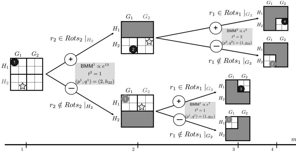
Figure 25.5 The tBMMF algorithm on the example from figure 25.4. Initially BP is run on the full matrix and is selected as the lowest-energy sequence. Rotamer is selected as the best max-marginal and used to partition the space in two. On the next iteration, BP is run on both subspaces to find the next lowest energy sequence (which we know contains ), and the best max-marginals from both spaces. We select because it has a higher max-marginal than . The space is partitioned again around and the third lowest-energy sequence contains . The next best max-marginal is , which we partition to find the fourth best energy sequence. Reprinted from [5].
over the marginals. In the initial state of the belief propagation iteration, each rotamer has the same probability, and every amino acid has a probability proportional to the number of rotamers. As the algorithm progresses through the states and messages are passed, the probability of each rotamer comes closer to the Boltzmann-weighted probability associated with low-energy states.
The method is very similar to what was described in section 25.7.2, but instead of max-product for messages as in equation (25.9), we use sum-product, which was previously introduced in section 25.3:
Sum-product is more appropriate for this problem because we are interested in more than just the single lowest-energy sequence. This is in contrast with section 25.7.2 where only the GMEC is of interest, and the max-product probabilities encode the GMEC.
Discussion and Future Directions
All the protein design algorithms described in this section (25.7) use Belief Propagation on models where the backbone is fixed and the side-chains are rigid. Kamisetty et al. [16] extend the free energy calculation of section 25.6 to include a limited number of sampled backbone conformations, based on the “backrub” motion. However, unlike MinDEE or BD (chapter 12), these algorithms lack the capability to model continuous flexibility in side-chains and backbones. Unlike backrub DEE (brDEE, chapter 12), which also uses discrete backbones, these BP techniques cannot guarantee identification of the GMEC or a gap-free enumeration of conformations in order of energy.
None of the algorithms presented in this chapter provides any guarantees on the results when the belief propagation step fails to converge; convergence is guaranteed only on tree graphs, which rarely occur in real protein design problems. Without provable convergence, we have no guarantee that we are generating the lowest-energy structures. If the BP design algorithms’ predictions fail to correlate with experimental results, the failure cannot be attributed with certainty to flaws in the input model (e.g., rotamer library, energy function, starting structure), since the inexactness of the BP method might have been responsible.
On the other hand, with a provable gap-free algorithm, any discrepancy between computational predictions and experimental results can be solely attributed to flaws in the model, and not to (for example) undersampling, or inadequate optimization. This makes it easier to feed back experimental results to improve the model. This capability is facilitated by modern statistical parameter estimation or machine learning algorithms. Indeed, one of the strengths of graphical models is that they can be constructed, or “learned” from experimental data [18]. Consider the situation where protein design is coupled with large-scale experimental screening. In this setting, false negatives (predictions that work well experimentally, but were predicted to perform poorly by the algorithm) may be observed. If the design algorithm is provable, then we know we can blame the model for these failures, and, in principle, improve it. This can be a tremendous advantage for a laboratory combining computational and experimental protein design. The tradeoff is that provable algorithms are frequently slower, require more computational resources, or are more complex to implement.
A promising approach is to use Belief Propagation to boost pruning and bounding in DEE/A*. Remarkably, this can be done while maintaining guarantees of completeness and soundness, using a deterministic algorithm. Hong et al. [9] observe the following: DEE methods combined with systematic A* search (DEE/A*) have proven useful, but may not be strong enough as we attempt to solve protein design problems where a large number of similar rotamers is eligible and the network of interactions between residues is dense. In the study [9], an exact solution method, named BroMAP (“branch-and-bound rotamer optimization using maximum a posteriori estimation”) is developed for protein design problems.
BroMAP is based on belief propagation, but the algorithm is provable and deterministic. BroMAP reduces the problem size within each node using DEE and pruning by lower bounds from approximate maximum a posteriori (MAP) estimation. The lower bounds are also exploited in branching and subproblem selection for fast discovery of strong upper bounds. BroMAP is able to expand smaller search trees than conventional branch-and-bound methods while performing only a moderate amount of computation in each node, thereby reducing the total running time. Computational results suggest that BroMAP tends to be faster than DEE/A* for large protein design cases. Therefore, BroMAP and other such belief propagation algorithms should be valuable for large protein design problems where DEE/A* struggles, and can also assist DEE/A* in GMEC search. Such algorithms represent the marriage of DEE and belief propagation, and are proving to be a powerful combination.
This chapter discussed only certain aspects of graphical models, Markov random fields, and belief propagation in computational structural biology. More generally, applications of belief propagation and graphical models include learning energy functions, side-chain packing, protein design, and NMR resonance assignment. These problems have been addressed in a number of recent papers [17, 9, 3, 4, 5, 6, 18, 23].
References
- [1] S.M. Aji and R.J. McEliece. The generalized distributive law and free energy minimization. Proceedings of the 39th Allerton Conference on Communication, Control and Computing (2003):459–467.
- [2] C.Y. Chen, I. Georgiev, A.C. Anderson, and B.R. Donald. Computational structure-based redesign of enzyme activity. Proceedings of the National Academy Science (U S A) 106;10(2009 Mar 10):3764-3769. Epub 2009 Feb 19.
- [3] M. Fromer and J.M. Shifman. Tradeoff between stability and multispecificity in the design of promiscuous proteins. PLoS Computational Biology 5;12(2009 Dec):e1000627. Epub 2009 Dec 24.
- [4] M. Fromer, C. Yanover, and M. Linial. Design of multispecific protein sequences using probabilistic graphical modeling. Proteins 78;3(2010 Feb 15):530–547.
- [5] M. Fromer and C. Yanover. Accurate prediction for atomic-level protein design and its application in diversifying the near-optimal sequence space. Proteins 75;3(2009 May 15):682–705.
- [6] M. Fromer and C. Yanover. A computational framework to empower probabilistic protein design. Bioinformatics 24;13(2008 Jul 1):i214-222.
- [7] I. Georgiev, R. H. Lilien, and B. R. Donald. Improved pruning algorithms and divide-and-conquer strategies for dead-end elimination, with application to protein design. Bioinformatics 22(2006 Jul):e174-183
- [8] I. Georgiev, R. H. Lilien, and B. R. Donald. The minimized dead-end elimination criterion and its application to protein redesign in a hybrid scoring and search algorithm for computing partition functions over molecular ensembles. Journal of Computational Chemistry 29;10(2008 Jul 30):1527–1542.
- [9] E. J. Hong, S. M. Lippow, B. Tidor, T. Lozano-Pérez. Rotamer optimization for protein design through MAP estimation and problem-size reduction. Journal of Computational Chemistry 30;12(2009 Sep):1923-1945.
- [10] X. Hu, H. Wang, H. Ke, and B. Kuhlman. High-resolution design of a protein loop. Proceedings of the National Academy of Sciences (U S A) 104;45(2007 Nov 6):17668-17673.
- [11] T. Lazaridis and M. Karplus. Effective energy functions for protein structure prediction. Current Opinion in Structural Biology 10(2000):138–145.
- [12] A. R. Leach and A. P. Lemon. Exploring the conformational space of protein side-chains using dead-end elimination and the A* algorithm. Proteins: Structure, Function, and Genetics 33(1998):227–239.
- [13] R. H. Lilien, B. W. Stevens, A. C. Anderson, and B. R. Donald. A novel ensemble-based scoring and search algorithm for protein redesign and its application to modify the substrate specificity of the gramicidin synthetase A phenylalanine adenylation enzyme. Journal of Computational Biology 12;6(2005 Jul-Aug):740–761.
- [14] P. D. Thomas and K. A. Dill. Statistical potentials extracted from protein structures: How accurate are they? Journal of Molecular Biology 257 (1996): 457–469.
- [15] H. Kamisetty, E. P. Xing, and C. J. Langmead. Free energy estimates of all-atom protein structures using generalized belief propagation. Journal of Computational Biology 15;7(2008 Sep):755–766.
- [16] H. Kamisetty, C. Bailey-Kellogg, and C. J. Langmead. A graphical model approach for predicting free energies of association for protein-protein interactions under backbone and side-chain flexibility. Proceedings of 3DSIG 2009 Structural Bioinformatics and Computational Biophysics (2009):67–68.
- [17] Y. Weiss and W. T. Freeman. Correctness of belief propagation in Gaussian graphical models of arbitrary topology. Neural Computation 13;10(2001 Oct):2173–2200.
- [18] C. Yanover, O. Schueler-Furman, and Y. Weiss. Minimizing and learning energy functions for side-chain prediction. Journal of Computational Biology 15;7(2008 Sep):899–911.
- [19] C. Yanover, M. Fromer, and J. M. Shifman Dead-end elimination for multistate protein design. Journal of Computational Chemistry 28(2007):2122–2129.
- [20] J. S. Yedidia, W. T. Freeman, and Y. Weiss. Understanding belief propagation and its generalizations, TR-2001-22. Mitsubishi Electric Research Laboratories, January 2002.
- [21] J. S. Yedidia, W. T. Freeman, and Y. Weiss. (2005) Constructing free-energy approximations and generalized belief propagation algorithms. IEEE Transactions on Information Theory 51;7(July 2005): 2282–2312.
- [22] J. S. Yedidia, W. T. Freeman, and Y. Weiss. Bethe free energy, Kikuchi approximations, and belief propagation algorithms, TR-2001-10. Mitsubishi Electric Research Laboratories, May 2001.
- [23] J. Zeng, P. Zhou, and B. R. Donald. A Markov random field framework for protein side-chain resonance assignment. Proceedings International Conference on Research in Computational Molecular Biology (RECOMB), 2010. Lisbon, Portugal.