Chapter 29Protein-Ligand NOE Matching
We return now to consider an application of graph algorithms to NMR and drug design. In this chapter, we describe protein-ligand “NOE matching,” a high-throughput method for binding pose evaluation that does not require protein NMR resonance assignments [1]. This chapter provides another example of the powerful Hungarian algorithm in computational structural biology.
Background
Determining binding pose is important in biochemistry, especially in drug design. However, for larger proteins, assigning resonances in proteins becomes much more difficult as spectra become much more cluttered, requiring a multitude of additional NMR experiments. An algorithm presented in Claus and coworkers [1] is called NOE matching, and addresses this problem, whose objective is to compute a protein-ligand binding pose without requiring protein NMR resonance assignments.
The data used in NOE matching is from three-dimensional (3D) -edited, -filtered HSQC-NOESY spectra, where only the NMR assignments of the bound ligand are essential. A 3D -edited, -filtered HSQC-NOESY, referred to as an 3D X-filtered NOESY, is the 3D combination of the HSQC with a NOESY experiment, which exploits the nuclear Overhauser effect (NOE). Simply, in an NOE, the resultant cross peak intensity measures the interatomic distance; heteronuclear single quantum correlation (HSQC) experiments record when two specific different types of atoms are covalently bound. The results of a 3D X-filtered NOESY experiment, as demonstrated in figure 29.1, can be represented as a 3D plot, where the - plane contains HSQC of a protein CH pair (with and frequencies of the protein being - and - axes, respectively), and the -axis showing the ligand frequency. The volume of peaks in the NOESY spectrum measure the distance between ligand and protein . Therefore, the 3D graph describes which protein CH pairs are near to which ligand H, and measures explicitly distances of ligand H’s to unassigned protein CHs.
Protein structure can often be determined through X-ray crystallography or be approximated reasonably well by homology modeling. In the work [1], the structures of the test cases come from crystallography, and the protein coordinates are from the Protein Data Bank (PDB). For our purposes, the most important feature of the X-filtered NOESY experiment is that by exploiting stable isotopic labeling, the pulse sequence ensures that all observed NOEs are intermolecular.
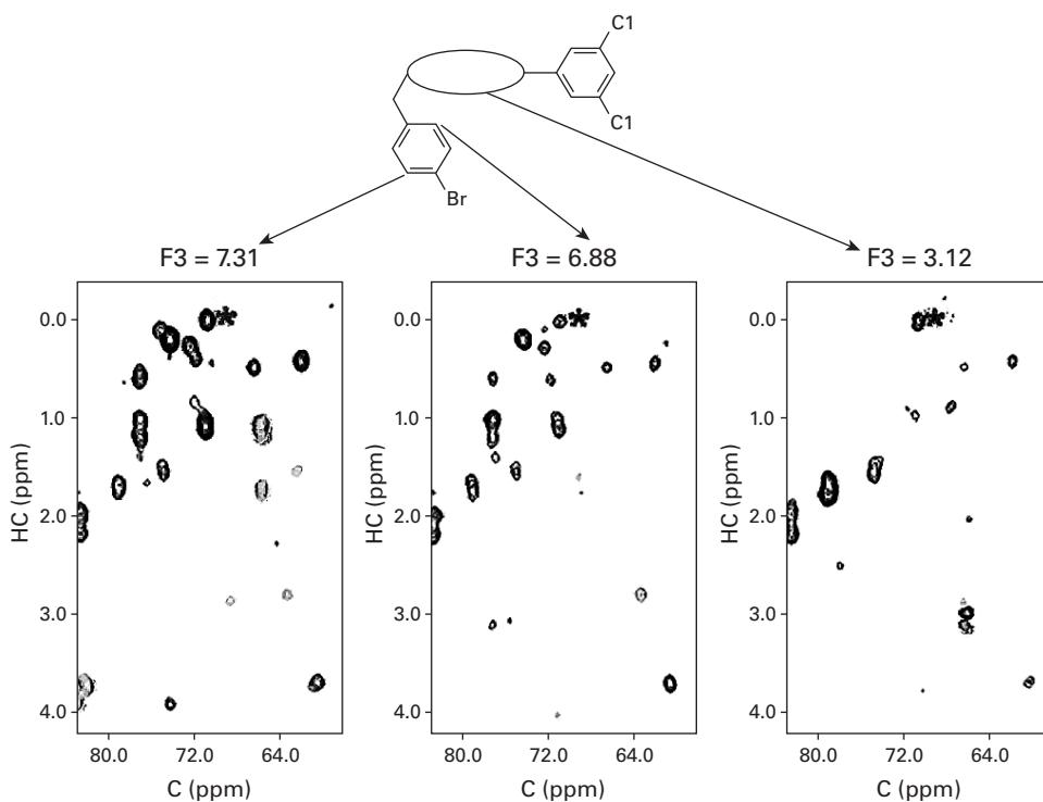
Figure 29.1 An example of an X-filtered NOESY spectrum, with the protein CH HSQC as the - plane, and the -axis (F3) referring to slices of the spectrum at the resonant frequencies of different ligand frequencies. Reprinted with permission. Copyright 2006 American Chemical Society. [1].
Methods
Claus and coworkers [1] determine the binding pose without protein resonance assignments. The recorded NOESY data is discretized according to signal strength, and compared with a back-calculated HSQC-NOESY spectrum based on a large, calculated ensemble of possible ligand poses. The computer-generated ligand pose whose synthetic NOESY spectrum is the best “match” with the experimental data, is assumed to be the correct binding pose. This NOE matching algorithm includes four steps:
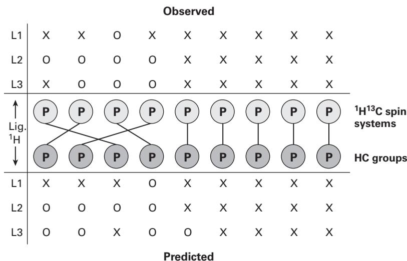
Figure 29.2 Equally partitioned bipartite graph representing a hypothetical instance of the 3D X-filtered NOESY bipartite graph-weighted matching problem, with [1]. Reprinted with permission. Copyright 2006 American Chemical Society.
Step 1. Trial Pose Generation Many trial poses are generated either using DOCK, or simulated annealing using the protein and the available trial poses of a similar ligand (with that ligand substituted for the compound of interest).
Step 2. Preparation of Experimental X-filtered NOESY Peak List The peaks of the experimental X-filtered NOESY are manually binned according to peak intensity from 1 to 4 (from least intense to most intense). Heuristic rules or higher-dimensional NMR experiments are used to determine peak shifts of the s.
Step 3. Prediction of Simulated X-filtered NOESY Spectra In a fast simulation, using the assigned ligand frequencies, distances from each ligand to every protein CH pair within 5 Å are classified as having intensity 1 to 4, referring to distances of 5 Å, 4 Å, 3 Å, and 2.5 Å, respectively. They are placed in the - plane using the mean chemical shifts of protein CH moieties available from the BioMagResBank. The algorithm is designed to “overpredict” peaks, such that there are more simulated peaks than experimental peaks.
Step 4. Spectrum Matching and Pose Scoring The predicted peaks are matched to the experimental peaks and a correlation score is generated. This is done using a variation of the bipartite graph-matching algorithm, as shown in figure 29.2. Each protein CH peak (considered a node in this graph) is separated into experimental and simulated vertices. Edge weights were determined by scoring the differences in peak intensities for each ligand ; this bipartite graph-matching problem is solved in time using the Hungarian algorithm, and poses are scored as the sum of the edge weights resulting from the optimization. A number of “unknown peak” nodes are generated as a place to store the worst-case matches of the simulated peaks.
The rules for determining edge weights are available in Claus and coworkers [1], but a global picture of these can easily be seen: There is no weight penalty for perfect matching of the intensity and the coordinates (within a margin of error), but the penalties are added as follows (in increasing order):
- Experimental peak and predicted peak of a different intensity. In a “loose” setting, this penalty obtains only if the difference is greater than 1; in a “tight” setting, all differences effect a small penalty.
- Simulated peak with no experimental peak, small penalty, since the algorithm aims to generate more simulated peaks than experimental.
- Experimental peak with no predicted peak, larger penalty.
This makes intuitive sense, since the algorithm essentially bins experimental peak intensities into four groups (allowing for small differences in intensity); likewise, the algorithm generates more simulated peaks than the experimental data, and therefore simulated peaks with no experimental peaks are not penalized as much as missing predicted peaks.
Results and Discussion
The results of the NOE matching algorithm are promising, as the authors observed a strong linear relationship between the cost of the pose and the RMSD to the experimentally determined binding poses, as shown in figure 29.3. More specifically, the average RMSD to the mean coordinates of ligand for the test case of mFABP/1 (muscle fatty acid–binding protein) is 0.42 Å, and that for the test case of LFA-1/2 (leukocyte function–associated antigen) is 0.19 Å.
Possible extensions to the algorithm include using this method as a fast filtering tool to eliminate poses that can definitely not be the binding pose, and using a higher-order CH frequency approximation based on quantum mechanical methods for a more accurate search on a smaller space. In addition to these, the study [1] suggests using more NMR experiments, which may be added to the algorithm, to more accurately assign resonances based on similarity to the generated data.
In conclusion, ‘NOE matching’ provides a fast filtering method for determining the binding poses of a ligand and protein, using minimal NMR data and with no need of protein resonance assignments. Although the paper [1] did not show any data for more difficult protein-ligand complexes, the results of the algorithm are accurate in the test cases reported.
Caveats In other applications, the Hungarian algorithm can be used reliably only when there is almost no noise in the edge weights. It would be interesting to evaluate the effect of noise on the performance of this application of the Hungarian algorithm. Can you design a more accurate matching algorithm?
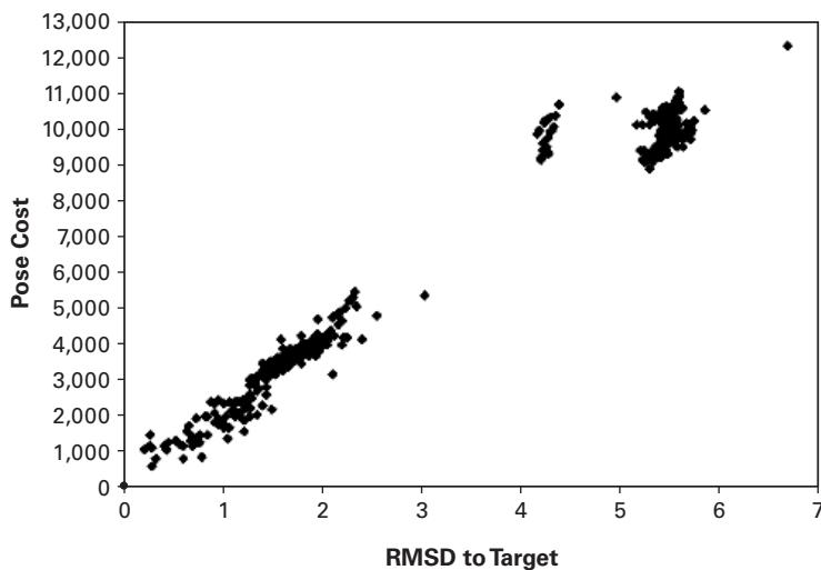
Figure 29.3 Costpose versus the RMSD (Å) to the target pose for mFABP/1 with synthetic (ideal) experimental and predicted 3D X-filtered NOESY data. This graph shows a fairly linear relationship. Reprinted with permission. Copyright 2006 American Chemical Society. [1].
Reference
[1] K. L. Constantine, M. E. Davis, W. J. Metzler, L. Mueller, and B. L. Claus. Protein-ligand NOE matching: A high-throughput method for binding pose evaluation that does not require protein NMR resonance assignments. Journal of the American Chemical Society 128;22(2006 Jun 7):7252–7263.