Chapter 31Distance Geometry
We now discuss, in several chapters, the theme of distance geometry, which relates to graph realization and NOE assignment. This topic touches on graph theory, algorithms, and topology, and is a classical and important subfield of computational structural biology.
The Molecule Problem
Consider a graph where is the set of atoms in a molecule. Attach an edge with weight between two vertices and if the distance between them is . This situation arises when we know the distance, either from empirical measurements such as NOEs, or from modeling (e.g., crystal structures of covalent bonds). The molecule problem is now the following. Given , can one compute the three-dimensional structure of the molecule? Formally, one wishes to construct a satisfying realization of the graph. A graph realization is an assignment of coordinates in to each vertex.
This problem could be formulated as a global optimization problem in the following way. Given a graph with weight over each edge , we are asked to assign a coordinate for each vertex , minimizing the following objective function:
where is the coordinate realization of vertex , is the distance between vertices and , and is the Euclidean norm. This objective function calculates the sum of squared deviations of the realized distances from the known distances. It will have a global minimum of zero when all the distance constraints are satisfied. The reason why the molecule problem is hard to solve in this form is that there are an exponential number of local minima. One approach to circumvent this problem is to break up the monolithic optimization problem into smaller problems and solve them independently. While this divide and conquer approach cannot always be applied to arbitrary optimization problems, Hendrickson [1, 2] shows it is possible for the molecule problem.
Divide and Conquer
The question is then, how can a divide and conquer approach be applied to the molecule problem? The answer lies in the observation that realized subgraphs can be combined to form larger realizations. Imagine that it were possible to split our graph into smaller subgraphs that are more easily realizable (this is sometimes possible, as we will see later). Each realization can then be treated as a rigid body and combined with other rigid bodies to form the final solution. We can find this solution by keeping one body fixed and searching the space of rotations and translations of the other bodies relative to the first. This search can be done with another global optimization step, but its success depends on the crucial assumption that each subgraph is uniquely realizable. That is, only one satisfying assignment of coordinates to the graph can exist. We then concern ourselves with partitioning our original graph in such a way that the subgraphs are uniquely realizable.
For this approach to work, we must make assumptions about the distances given. First, the distances must be known exactly. This is not feasible for real NOESY spectra, which reveals this work as somewhat of a theoretical exercise. However, these algorithms could be applied if exact distances could be inferred (or even measured directly) from molecules in the future. Moreover, it may be that solving a problem without noise or error in the data can provide insight into the real problem with experimental uncertainty. The second assumption is that the source of the distance constraints (which can also be viewed as a realization of ) must comprise a set of algebraically independent coordinates. That is, we need a generic realization. This means the original atom positions cannot satisfy any polynomial equation. An example of a configuration excluded by this requirement is when four or more atoms lie on the same plane. It may seem like a strong requirement of the data, but in practice, almost all realizations are generic.
Conditions for Unique Realizability
What properties does a graph need to be uniquely realizable? Hendrickson shows there are three conditions a graph must satisfy to have a unique realization in :
- vertex-connectivity;
- Redundant rigidity; and
- The stress matrix has nullity ().
Hendrickson also shows the first two conditions are necessary conditions and the third condition is sufficient.
Graph connectivity is a well-studied property of graphs and is not reviewed here. Redundant rigidity is a modification of the concept of graph rigidity (see chapter 21, section 21.2), which can be thought of as follows. Imagine if one were to physically pick up a graph with one’s hands and try to bend it. A rigid graph would not allow any motions (or flexings) but a flexible graph would. Figure 31.1 illustrates this concept.
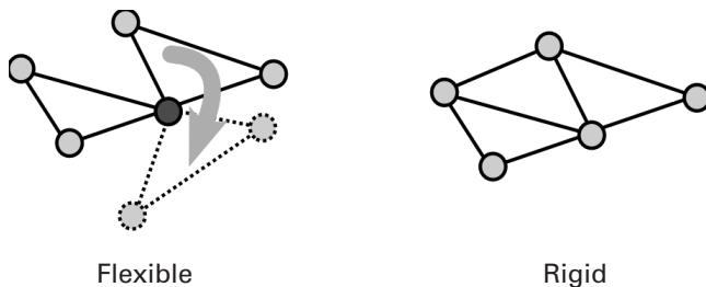
Figure 31.1 Flexible vs. Rigid graphs in . On the left, the graph is flexible because the right portion is free to rotate about the dark vertex. On the right, no such dark vertex could exist. Credit: Jeff Martin and Bruce Donald.
Redundant rigidity is then a property that describes a graph that remains rigid even after any single edge is removed.
To characterize the stress of a graph, we turn to mechanical engineering and static systems. If one were to view a graph as a bridge, the edges could become steel beams and the vertices could become joints. It is often useful to calculate the equilibrium of such a system. To do this, we assign weights to each edge. Then we are interested in finding values for the weights such that, for any vertex, the weighted sum of all the edge vectors starting from this vertex is zero. This weight that we assigned is called a stress of the graph. The stress itself is a scalar quantity, but the direction of the edge it describes can give it a vector interpretation. It is the sum of these stress vectors, then, that we wish to be zero and not the stresses directly. Let be the stress of an edge . The equilibrium condition is then
for all where, again, is the position of vertex in . We can then construct the stress matrix
and examine its nullity to determine unique realizability.
Graph Partitioning
Once we know conditions for uniquely realizable graphs, we then turn to partitioning a graph such that the subgraphs satisfy those conditions. Again, vertex connectivity is a well-studied problem and efficient algorithms exist for partitioning graphs in that sense. One challenge Hendrickson addresses is how to partition graphs so that their subgraphs are redundantly rigid. His algorithm is based on the following intuition. An edge that is not redundant in the whole graph cannot be redundant in any subgraph. Therefore, one can remove such a nonredundant edge from the graph and examine its flexibility. Regions of the graph that are not flexible can then be targeted for subgraph partitioning.
A related problem is that, in the preceding case, we were interested in finding the maximal subgraphs that were still redundantly rigid; however, sometimes these maximal graphs are still too large for feasible processing. In this case, we want to further break up the graph and, in practice, Hendrickson found the optimal subgraph size to be 15 vertices. If it is any smaller, the divide and conquer approach would spend more computational time on the merge step; any larger, and solving the realization problem on the subgraph would become more difficult. Graphs can be broken up by finding a vertex separator. Then two graph pieces will have a number of vertices in common, which will simplify the recombination of their realizations later in the merge step.
Once graphs are found that pass both of the first two conditions (section 31.3), the algorithm checks for the third condition. Note that the algorithm has no recourse for subgraphs that do not pass the third condition. Hendrickson states that in , no such graph is known that satisfies the first two conditions and not the third. Were such a graph to be found, Hendrickson instructed the algorithm to return it so he could study its properties.
Realizing Subgraphs
Finally, to realize these subgraphs, we formulate the problem as a global optimization (similar to the one described in section 31.1). Up until this point, we have focused on reducing the complexity of the realization problem while still preserving the guarantee that our answer is correct. This is because we must rely on a global optimization to perform the actual realization step. The distance geometry problem has been proven to be strongly NP-hard [3], so the cost of performing the optimization is high even for much smaller problems. Therefore, Hendrickson makes every effort to minimize the complexity of the optimization problem before relying on the optimizer to compute the answer.
Hendrickson also uses another intuition to simplify realization. Imagine a set of four vertices have already been realized in . Then, to completely specify the position of a fifth vertex, one merely needs distances to the four already-realized vertices. One can then “grow” the chunk of realized vertices by attaching other vertices given an adequate number of distance restraints. In this context, “chunk” refers to a connected group of realized vertices. This part of the realization process can be accomplished combinatorially for a relatively low cost compared to optimization. Thus, by realizing chunks or “easy bits” of the graph first, the final problem that must be ultimately optimized is greatly simplified. Finally, the optimization problem concerns itself with the task of fixing an arbitrary chunk and trying to find the positions of other chunks that satisfy the distance restraints completely. Once the subgraphs are realized, we can merge them in the same way by using the optimizer. Once all realizations are successfully merged, we can then know the full structure of the “protein” whose geometry the graph encodes.
Conclusion
Hendrickson states that his approach requires exact interatomic distances to correctly solve the protein structure. He also states that the algorithm is intolerant to noisy or miscalculated restraints. While this removes some of the immediate applicability for solving structures, it does lay theoretical groundwork for future work in the area.
In some cases, there may simply not be enough distance restraints to completely specify the full structure of a protein. This could be a catastrophic input for some algorithms that assume complete data. However, Hendrickson’s divide and conquer approach allows his algorithm to recurse on subgraphs and solve them independently. In some cases, this subgraph might correspond to a meaningful region of the protein such as a binding site or a particular functional domain. Conversely, the absence of redundant rigidity might give evidence that the protein is flexible or that more experiments are required to define the native structure.
References
- [1] B. Hendrickson. The molecule problem: Exploiting structure in global optimization. SIAM Journal of Computing 5;4(November 1995):835–857.
- [2] B. Hendrickson. Conditions for unique graph realizations. SIAM Journal of Computing 21;1(February 1992):65–84.
- [3] J. B. Saxe. Embeddability of weighted graphs in k-space is strongly NP-hard. Tech. Report, Computer Science Department, Carnegie-Mellon University, Pittsburgh, PA, 1979.