Chapter 37Graph Cuts for Energy Minimization and Assignment Problems
Graph cuts have numerous applications in computational structural biology. In this chapter, we introduce a generalized Potts energy model in the Markov Random Field (MRF) framework, and present a multiway graph cut algorithm to find the minimum energy [1]. Then, we present an -expansion move algorithm to compute visual correspondence with occlusions [2]. Graph cuts provide an algorithm for a wide variety of assignment problems.
Some of these assignment problems first arose in machine vision. We review these vision problems since image processing arises often in computational biology. However, graph cuts also have broader applications, as we shall see. This chapter builds on the MRF concepts introduced in chapter 25.
Construction of the Energy Function
Markov Random Fields (MRFs) An image is an array of pixels connected in a grid topology. Suppose that we are given two images. A pixel in one image is said to correspond to a pixel in the other if these two pixels are projections along lines of sight from the same physical scene element [2]. In the visual correspondence problem, we can regard the pixels in the second image as labels, and our goal is to compute a “label” , which denotes a disparity value, for each pixel in the primary image. Let denote the disparity at pixel , and denote the set of the neighbors of . In a Markov Random Field (MRF) framework, we have
Hammersley-Clifford Theorem Let denote a configuration of all pixels . If we focus on the MRF framework, with a clique potential , we have
where denotes the observed data. By Bayes’ rule, we have
where is also called the posterior probability; is the prior probability, obtained from equation (37.1), and is called the likelihood probability,1 which also represents the sensor noise model.
Energy Minimization We wish to find a configuration that minimizes the posterior energy function:
The Generalized Potts Model In a Generalized Potts Model MRF (GPM-MRF), a clique potential for any pair of neighboring pixels and is defined by
where if , otherwise, and denotes the penalty for discontinuity at pair . The posterior energy function of a GPM-MRF is
Optimizing the Energy Function by Graph Cuts
Graph Construction
Given a set of pixels and a set of labels , we construct a graph such that and the edge set is constructed in the following way. Any two neighboring vertices in are connected by an edge, called an -link. Each -link between pixels and is assigned a weight:
A vertex in is connected to a vertex in if . Each edge is called -link, which is assigned a weight:
where denotes some constant for each pixel .
1 Here, is the sensor noise distribution.
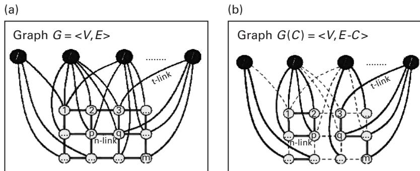
Figure 37.1 (plate 41)
An example of multiway graph cut. Dashed lines in (b) denote the cut edges in the graph [1]. Copyright 1998 IEEE.
Figure 37.1a shows an example of such a constructed graph.
The Multiway Cut Formulation
A subset of edges in a graph is a multiway cut if the terminals (label vertices) are separated in the induced graph . Figure 37.1 (plate 41) shows a multiway cut example in a graph. The cost of a cut , denoted by , is equal to the sum of weights of all cut edges. The multiway cut problem is to find a multiway cut with the minimum cost.
Theorem If is a multiway cut with the minimum cost, then the corresponding configuration (see section 37.3.3) minimizes in equation (37.3).
The Multiway Cut Algorithm
A special case of the multiway cut problem, in which there are only two terminals, is a standard min-cut problem and can be solved in polynomial time using the max-flow (Ford-Fulkerson) algorithm. The general multiway cut problem in which there are more than two labels is NP-complete. Currently, efficient approximation algorithms exist that are optimal within a factor of 2. The following algorithm (algorithm 1) is applied to find the minimum cut for a given graph:
Algorithm 1
- 1: Start with an arbitrary multiway cut from any pair of terminals.
- 2: while improves do
- 3: for all pairs of labels and do
- 4: Find min cut on .
- 5: Update if a better new cut is found.
- 6: end for
- 7: end while
- 8: Return .
Graph Cuts for Computing Visual Correspondence with Occlusions
Notation
Computing Visual Correspondence Suppose that we are given two images. A pixel in one image is said to correspond to a pixel in the other if these two pixels are projections along lines of sight from the same physical scene element [2]. In the visual correspondence problem, we can regard the pixels in the second image as labels, and our goal is to compute a “label” , which denotes a disparity value, for each pixel in the primary image. In other words, the visual correspondence problem can be formulated into a GPM-MRF. The reader is referred to section 4 in Boykov et al. [1] for more implementation details.
Occlusion Problem In a visual correspondence problem, some pixels may be visible only in one image, but occluded in the other one. Hence, there is no correspondence for these pixels (or “labels”) in the other image.
-Expansion Move Let denote the disparity of an assignment . In an -expansion move operation, some currently active assignments are deleted, and some assignments with disparity are added.
Energy Function
The basic idea of designing the energy function here is to construct an energy model on assignments so that the graph cut algorithms can be applied. Here each vertex in a graph represents an assignment between two corresponding pixels, while in the previous section (37.2), each vertex in the graph denotes a pixel in the image.
Given a configuration of pixel assignments (or correspondences) between two images, the energy function incorporating the occlusion correspondences is defined by
where denotes the intensity difference between corresponding pixels, and denotes a penalty for an occluded pixel, and denotes a smoothness between two neighboring assignments. More specifically, these three terms are designed as follows (we use the same terminology as in section 3.2 from Kolmogorov and Zabih [2]):
- , where denotes the disparity of an assignment , and denotes the intensity of pixel .
- , where denotes a penalty if pixel is occluded, and denotes the set of active assignments involving pixel , and is 1 if its argument is true, and 0 otherwise.
- , where denotes the neighborhood system.
- Start with an arbitrary unique configuration
- Set success
- For each disparity
- 3.1. Find among unique within single -expansion of
- 3.2. If , set and success
- If success = 1 goto 2
- Return
Figure 37.2 The -expansion move algorithm [2].
The -Expansion Move Algorithm
Overview of the Algorithm The algorithm to find the configuration with the minimum energy is described in figure 37.2. The key step in the expansion algorithm is to find the configuration with smallest energy within a single -expansion move. This step is implemented by constructing a weighted graph such that the minimum graph cut is equal to the configuration with the minimum energy. The following section shows how to construct the desired graph and compute the minimum cut.
Graph Construction Let denote the starting configuration. Let denote the set of all possible assignments within one -expansion move, where and . Now we construct a directed graph where nodes are all assignments in plus two terminal nodes and , and edges are constructed according to the following rules:
- For every vertex , edges and are constructed.
- Edges and are constructed if .
- Edges exist between assignments and , where .
Figure 37.3 shows an example of a constructed graph. The weights assigned for all edges are shown in table 37.1.
Graph Cuts Given a cut on , the configuration corresponding to the cut is defined by
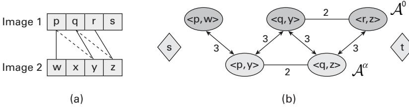
Figure 37.3 An example of a constructed graph to find the minimum energy within one -expansion move. (a) and denote two original images. Solid lines represent the current active assignments, and dashed lines represent the assignments after an -expansion move (here ). (b) Vertices in the top row represent the assignments in set , and vertices in the bottom row represent the assignments in . The number associated with each edge represents the rule order applied. The edges from rule 1 are not shown here [2]. Copyright 2001 IEEE.
Table 37.1 Assigned weights for all edges [2]
| Edge | Weight | For |
|---|---|---|
The following theorem shows that the minimum cut of a constructed graph is equal to the unique configuration with the minimum energy within one -expansion move.
Theorem [2] Let be the minimum cut on . Then is the unique configuration that minimizes the energy within one -expansion move of .
The minimum cut of the graph can be computed by using the Ford-Fulkerson algorithm in polynomial time.
Comments What is the difference between the graph cut algorithm and the other methods for assignment, such as the EM or bipartite matching approach?
Exercise The pixel assignment problem can be generalized to the NMR resonance and NOE assignment problems by first generalizing the grid network to have a more general graph neighborhood topology. What is the best algorithm you can obtain for these NMR problems? Analyze the complexity of your algorithm. Compare to EM and bipartite matching. Will graph cuts be more, or less robust than bipartite matching? Explain. Implement and test your algorithm, using both synthetic and real NMR data.
References
- [1] Yuri Boykov, Olga Veksler, Ramin Zabih. Markov Random fields with efficient approximations. Proceedings of IEEE Conference on Computer Vision and Pattern Recognition (CVPR) (1998). Santa Barbara, CA.
- [2] V. Kolmogorov and R. Zabih. Computing visual correspondence with occlusions using graph cuts. Proceedings of the Eighth International Conference on Computer Vision (ICCV-01) 2001, Vancover, British Columbia.