Chapter 39Protein Unfolding by Using Residual Dipolar Couplings
This chapter discusses ensemble-based computational models for unfolded proteins, and evaluates the effectiveness of these models by comparing the ensemble-averaged residual dipolar couplings (RDCs) and small-angle X-ray scattering (SAXS) data [2, 1].
Motivation and Overview
Natively unfolded regions have been shown to be common in functional proteins in a vast range of biochemical processes. In contrast to classical structural biology, unfolded proteins must be described by an ensemble of intermediate conformers. Many “traditional” NMR experiments, which have been widely used for structure determination in classical structural biology, are still feasible for the study of unstructured (or “intrinsically disordered”) proteins in solution, since the NMR experimental data, such as chemical shifts and residual dipolar couplings (RDCs), can still be measured in highly disordered states, and thus used to characterize average properties over the ensemble of conformers. See chapter 7.
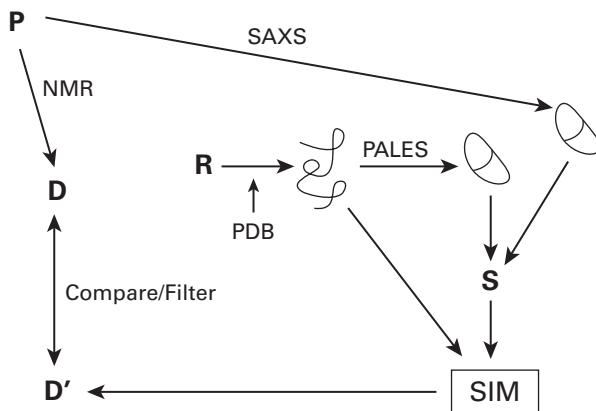
The methodology applied by Bernado et al. [1, 2] is shown in figure 39.1.
Ensemble Computation Using Only Local Sampling
We now give an algorithm to compute the conformational ensemble based only on local sampling of backbone dihedral angles, and then compare the computed ensemble-averaged RDCs with experimental data.
The algorithm [1] generates a statistical ensemble of conformations and calculates the average RDCs over the whole ensemble:
- Local random sampling of angles Build sequential peptide chains using randomly chosen angles from a database of amino acid–specific conformations, which are obtained from loop regions of high-resolution X-ray structures.
- Steric clash checking For each residue, check whether it has steric clash with another residue in the chain, or with the invariant folded fragment. The pair with steric overlap is rejected,
P = Protein
D = Expt RDCs
D’ = Back-calculated RDCs
R = Random / MC sampling
= Computed structure
= Ellipsoid (hydrodynamic ratio or SAXS data)
S = Saupe matrix and a new angle is randomly selected until no overlap occurs. In total, feasible conformers are generated.
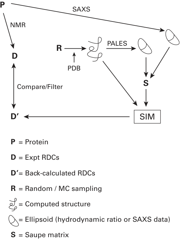
Figure 39.1 Overview of methodology. The module SIM computes the ensemble average of the back-calculated RDCs, given a set of structures.
3. Ensemble-average RDC computing The alignment tensor for each complete conformer is first predicted based on the hydrodynamic shape. Then each RDC associated with a corresponding NH vector with respect to this tensor is back-computed (simulated). RDCs from each NH bond are averaged over all conformers.
Figure 39.2 (plate 42) shows comparisons between the ensemble-average (simulated) and experimental RDCs for the S protein ( S stands for alpha-synuclein). The computed ensemble-averaged RDCs fit the experimental data well in the central regions (residues 30–110), but there are significant deviations in the N-and C-terminal regions.
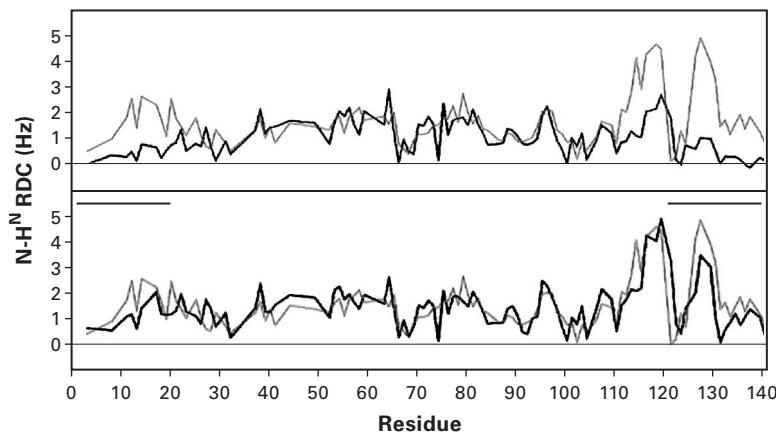
Figure 39.2 (plate 42)
Comparisons between ensemble-averaged RDCs (red) simulated without long-range contacts, and experimental RDCs (blue) for protein S in (a) Pf1 bacteriophage and (b) lyotropic media. Simulated data are scaled to maximize fit in the region 22–112. For illustration purposes, the RDC sign is inverted compared to the usual conventions [1]. Reprinted with permission. Copyright 2005 American Chemical Society.
Ensemble Computation with Both Local Sampling and Long-Range Order
The ensemble computation by incorporating the long-range contacts between the N-and C-terminal domains improves the agreement between simulated and experimental RDCs.
The algorithm is similar to that in section 39.4.2 except that a new step is added to model the long-range contacts. The following shows the modified algorithm:
- Local random sampling of ( , ) angles Similar to the corresponding step in section 39.2.
- Steric clash checking Similar to the corresponding step in section 39.2.
- Conformer selection based on long-range contacts The primary sequence is divided into several fragments, and two fragment positions are specified. When there is a long-range contact, each generated conformer is accepted only when a atom at one specified fragment position is less than 15 Å from a atom in the other specified domain.
- Ensemble-average RDC computing Similar to the corresponding step in section 39.2.
Figure 39.3 shows the differences between experimental and simulated RDCs for protein S incorporating long-range contacts. In figure 39.3e (plate 43), the distribution of experimental RDCs closely agrees with that of simulated RDCs when the long-range contacts between the N-and C-terminal regions (residues 1–20 and 121–140) are considered.
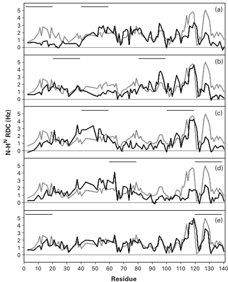
Figure 39.3 (plate 43) Comparisons between experimental (blue) and simulated RDCs incorporating the long-range contacts (red). Contact regions are indicated by bars. (a) (1–20, 41–60); (b) (21–40, 81–100); (c) (41–60, 101–120); (d) (61–80, 121–140); (e) (1–20, 121–140) [1].
An Unfolded Protein Structure Model from RDCs and Small-Angle X-Ray Scattering (SAXS) Data
Generation of the Conformation Ensemble
We can generate the conformational ensemble of disordered regions of proteins by using a similar approach as in section 39.2, except that here we need to determine the first peptide unit position in the unfolded domain.
Determination of the First Peptide Unit in the Unfolded Domain The orientation of the first peptide unit may be inconsistent with the relative orientations of folded domains. Thus, it is necessary to find the optimal orientation of the first peptide plane. In Bernado et al. [2], the first peptide plane is rotated over a grid on , until the alignment tensor frames of the folded and unfolded domains are consistent with each other. The correct orientation of the first peptide plane is used to compute each new ensemble. Compare chapters 13, and 17, sections 17.2 and 17.3.
RDC Computation from the Conformational Ensemble
Prediction of the Alignment Tensor The alignment tensor for each conformer is calculated by exploiting the similarity between the alignment and the radius of gyration. The shape of the RDC distribution (or a similar property comparable to the radius of gyration), denoted by , can be regarded as a function of the alignment tensor. We must search for an alignment tensor such that the computed fits the radius of gyration well. Based on the alignment tensor and the generated structure, the RDCs for each conformer can be computed. Compare chapters 13, 14.
Figure 39.4 (plate 44) shows the comparisons between simulated (ensemble-averaged) and experimental RDCs for protein PX. The RDC distribution, obtained from the ensemble computed from the above scheme, has good agreement with the distribution of experimental RDCs.
Prediction of SAXS Data from the Conformational Ensemble
SAXS data gives the radius of gyration of the protein, and is related to a size and shape of a molecular system. SAXS data may be back-computed as follows. First, side-chains are added to the unfolded domains using the SCCOMP program, and then the SAXS intensities are predicted using the CRYSOL program. After that, the radius of gyration is calculated from the predicted SAXS intensities based on the Debye equation [2].
Figure 39.5 shows the difference between simulated and experimental SAXS data. We see that the size and shape of the ensemble reproduce the SAXS data for the unfolded domains.
Protein Backbone Structure Determination Using Only RDCs The following sketches the algorithm [3] to compute the protein backbone structure using only RDCs. A variation of this algorithm was used in the protein unfolding work described in the first part of this chapter.
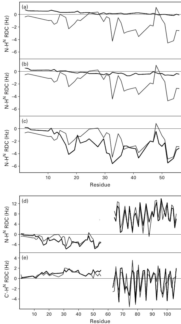
Figure 39.4 (plate 44) Comparison between simulated (red) and experimental (blue) RDCs for protein PX. PX is numbered from 1 to 109 and contains the 14-residue His tag, such that residues 15–109 correspond to the region 474–568 in the intact C-terminal domain protein. (a) Experimental N-HN RDCs compared with RDCs simulated in the unfolded domain of PX using random sampling of backbone dihedral angle ( ) space. In this model, (1) no nonbonded interactions were taken
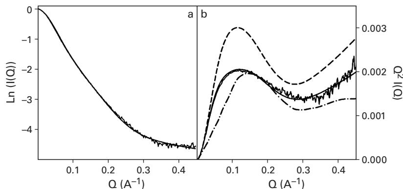
Figure 39.5 Comparisons between simulated and experimental SAXS data for protein PX. (a) Comparison of background corrected experimental SAXS data [intensity ] versus scattering vector with the simulated scattering curves averaged over the ensemble. The curves were normalized by dividing all intensities by the value of extracted from fitting to the Debye relationship. (b) Comparison of Kratky plots where is plotted against the scattering vector . This representation of the data is sensitive to the overall shape of the scattering object and in this case to the relative dimensions of the folded and unfolded domains. Experimental data (gray) are shown in comparison to ensembles calculated by using model III with the native sequence (solid line), a polyglycine sequence (dashed line), and a sequence where the distributions are located in the extended region of the Ramachandran plot (dashed-point line) [2]. Copyright 2005 National Academy of Sciences.
- Alignment Tensor Prediction The RDC for a known bond vector in the frame of alignment tensor can be computed by . We must find an alignment tensor such that the following target function is minimized:
where and represent the experimental and computed RDCs.
- Computation of Angles The RDCs in two media can restrict the orientation of each bond vector to a discrete and finite solution space (see chapters 15–18). The paper [3] uses the chiral motif, that is, bond vectors - , - , to filter out ambiguous peptide plane orientations. In cases when some RDCs are missing, the optimal angles are found using a stochastic search such that all other relevant vector orientations are satisfied.
into account except for avoiding overlap between the folded and unfolded domains. This model is essentially a random flight chain model of the polymer and reproduced the expected bell-shaped distribution along the chain. (b) Experimental N-HN RDCs compared with RDCs simulated in the unfolded domain of PX using random sampling of backbone dihedral angle space. In this model (II) nonbonded interactions between residues in the unfolded domain were taken into account by using a simple steric repulsion model. Overlap between the folded and unfolded domains was also avoided. (c) Experimental N-HN RDCs compared with RDCs simulated in the unfolded domain of PX using random sampling residue-specific propensities found in loop regions of a database of folded proteins combined with the simple volume exclusion model (model III). (d) Simulated and experimental N-HN RDCs from the entire protein by using model III. (e) Simulated and experimental C’-HN RDCs from the entire protein using model III [2]. Copyright 2005 National Academy of Sciences.
Notes Since RDCs represent global orientational constraints, the regions where little or no data is available do not propagate to introduce errors in other regions of the backbone.
Exercise Compare the approach in Hus et al. [3] to RDC-EXACT (chapters 15–18). The algorithm in [3] is called Meccano. Explain how Meccano can be extended or modified to obtain a provable algorithm.
Exercise Compare the algorithm in this chapter to the technique in chapter 7. Contrast the methods, and discuss the similarities and differences.
References
- [1] P. Bernado, C. W. Bertoncini, C. Griesinger, M. Zweckstetter, and M. Blackledge. Defining long-range order and local disorder in native alpha-synuclein using residual dipolar couplings. Journal of the American Chemical Society 127;51 (2005 Dec 28):17968–17969.
- [2] P. Bernado, L. Blanchard, P. Timmins, D. Marion, R. W. Ruigrok, and M. Blackledge. A structural model for unfolded proteins from residual dipolar couplings and small-angle x-ray scattering. Proceedings of the National Academy of Science U S A 102;47 (2005 Nov 22):17002–17007.
- [3] Jean-Christophe Hus, Dominique Marion, and Martin Blackledge. Determination of protein backbone structure using only residual dipolar couplings. Journal of the American Chemical Society 123 (2001): 1541–1542.