Appendix BMaking Sense of Data: A Statistics Primer
This appendix is designed help you understand the analysis of biological data in a statistical context. We outline major concepts involved in the collection and analysis of data, and we present basic statistical analyses that will help you interpret, understand, and complete the problems throughout this book as well as understand and interpret scientific studies in general. We present formulas for some common statistical tests as examples, but the main purpose of this appendix is to help you understand the purpose and reasoning behind statistical tests. Once you understand the basis of an analysis, you may wish to use one of many free, online websites for conducting the tests (such as http://vassarstats.net).
Why Do We Need Statistical Analysis?
ALMOST EVERYTHING VARIES We live in a variable world, but within the variation we see among biological organisms there are predictable patterns. We use concepts and methods from the field of statistics to find and analyze these patterns. Consider any group of common things in nature—all women aged 22, all the cells in your liver, or all the blades of grass in your yard. Although they will have many similar characteristics, they will also have important differences. Men aged 22 tend to be taller than women aged 22, but of course not every man will be taller than every woman in this age group.
Natural variation can make it difficult to find general patterns. For example, scientists have determined that smoking increases the risk of getting lung cancer. But we know that not all smokers will develop lung cancer and not all nonsmokers will remain cancer-free. If we compare just one smoker with just one nonsmoker, we may end up drawing the wrong conclusion. So how did scientists discover this general pattern? How many smokers and nonsmokers did they examine before they felt confident about the risk of smoking?
Statistics helps us detect and describe general patterns in nature, and draw conclusions from those patterns.
AVOIDING FALSE POSITIVES AND FALSE NEGATIVES When a woman takes a pregnancy test, there is some chance that it will be positive even if she is not pregnant, and there is some chance that it will be negative even if she is pregnant. We call these kinds of mistakes “false positives” and “false negatives.”
Doing science is a bit like taking a medical test. We observe patterns in the world, and we try to draw conclusions about how the world works from those observations. Sometimes our observations lead us to draw the wrong conclusions. We might conclude that a phenomenon occurs, when it actually does not; or we might conclude that a phenomenon does not occur, when it actually does.
For example, planet Earth has been warming over the past century (see Key Concept 56.4). Ecologists are interested in whether plant and animal populations have been affected by global warming. If we have long-term information about the locations of species and about temperatures in certain areas, we can determine whether shifts in species distributions coincide with temperature changes. Such information, however, can be very complicated. Without proper statistical methods, one may not be able to detect the true impact of temperature, or instead may think a pattern exists when it does not.
Statistics helps us avoid drawing the wrong conclusions.
How Does Statistical Analysis Help Us Understand the Natural World?
Statistical analysis is essential to scientific discovery. Most biological studies involve five basic steps, each of which involves aspects of statistical analysis.
- Step 1: Experimental Design Clearly define the scientific question and the methods necessary to tackle the question.
- Step 2: Data Collection Gather information about the natural world through observations and experiments.
- Step 3: Organize and Visualize the Data Use tables, graphs, and other useful representations to gain intuition about patterns in the data.
- Step 4: Summarize the Data Summarize the data with a few key statistical calculations.
- Step 5: Inferential Statistics Use statistical methods to draw general conclusions from the data about the world and the ways it works.
Step 1: Experimental Design
We make observations and conduct experiments to gain knowledge about the world. Scientists come up with scientific ideas based on prior research and their own observations. These ideas start as a question such as “Does smoking cause cancer?” From prior experience, scientists then propose possible answers to the question in the form of hypotheses such as “Smoking increases the risk of cancer.” Experimental design then involves devising comparisons that can test predictions of the hypotheses. For example, if we are interested in evaluating the hypothesis that smoking increases cancer risk, we might decide to compare the incidence of cancer in nonsmokers and smokers. Our hypothesis would predict that the cancer incidence is higher in smokers than in nonsmokers. There are various ways we could make that comparison. We could compare the smoking history of people newly diagnosed with cancer with that of people whose tests came out negative for cancer. Alternatively, we could assess the current smoking habits of a sample of people and see whether those who smoke more heavily are more likely to develop cancer in, say, 5 years. Statistics provides us with tools for assessing which approach will provide us with an answer with smaller costs in time and effort in data collection and analysis.
We use statistics to guide us in planning exactly how to make our comparisons—what kinds of data and how many observations we will need to collect.
Step 2: Data Collection
TAKING SAMPLES When biologists gather information about the natural world, they typically collect representative pieces of information, called data or observations. For example, when evaluating the efficacy of a candidate drug for medulloblastoma brain cancer, scientists may test the drug on tens or hundreds of patients, and then draw conclusions about its efficacy for all patients with these tumors. Similarly, scientists studying the relationship between body weight and clutch size (number of eggs) for female spiders of a particular species may examine tens to hundreds of spiders to make their conclusions.
We use the expression “sampling from a population” to describe this general method of taking representative pieces of information from the system under investigation (Figure B1). The pieces of information together make up a sample of the larger system, or population. In the cancer therapy example, each observation was the change in a patient’s tumor size 6 months after initiating treatment, and the population of interest was all individuals with medulloblastoma tumors. In the spider example, each observation was a pair of measurements—body weight and clutch size—for a single female spider, and the population of interest was all female spiders of this species.
Sampling is a matter of necessity, not laziness. We cannot hope (and would not want) to collect and weigh all of the female spiders of the species of interest on Earth! Instead, we use statistics to determine how many spiders we must collect to confidently infer something about the general population and then use statistics again to make such inferences.
DATA COME IN ALL SHAPES AND SIZES In statistics we use the word “variable” to mean a measurable characteristic of an individual component of a system. Some variables are on a numerical scale, such as the daily high temperature or the clutch size of a spider. We call these quantitative variables. Quantitative variables that take on only whole number values (such as spider clutch size) are called discrete variables, whereas variables that can also take on a fractional value (such as temperature) are called continuous variables.
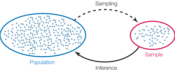
Figure B1 Sampling from a Population Biologists take representative samples from a population, use descriptive statistics to characterize their samples, and then use inferential statistics to draw conclusions about the original population.
Other variables take categories as values, such as a human blood type (A, B, AB, or O) or an ant caste (queen, worker, or male). We call these categorical variables. Categorical variables with a natural ordering, such as a final grade in Introductory Biology (A, B, C, D, or F), are called ordinal variables.
Each class of variables comes with its own set of statistical methods. We will introduce a few common methods in this appendix that will help you work on the problems presented in this book, but you should consult a biostatistics textbook for more advanced tests and analyses for other data sets and problems.
Step 3: Organize and Visualize the Data
Your data consist of a series of values of the variable or variables of interest, each from a separate observation. For example, Table B1 shows the weight and length of 34 fish (Abramis brama) from Lake Laengelmavesi in Finland. From this list of numbers, it’s hard to get a sense of how big the fish in the lake are, or how variable
Table B1 Weight and Length Measurements for a Sample of Abramis brama from Lake Laengelmavesi
| Individual number | Fish weight (g) | Fish length (cm) |
|---|---|---|
| 1 | 242 | 30.0 |
| 2 | 290 | 31.2 |
| 3 | 340 | 31.1 |
| 4 | 363 | 33.5 |
| 5 | 390 | 35.0 |
| 6 | 430 | 34.0 |
| 7 | 450 | 34.7 |
| 8 | 450 | 35.1 |
| 9 | 475 | 36.2 |
| 10 | 500 | 34.5 |
| 11 | 500 | 36.2 |
| 12 | 500 | 36.2 |
| 13 | 500 | 36.4 |
| 14 | 575 | 38.7 |
| 15 | 600 | 37.3 |
| 16 | 600 | 37.2 |
| 17 | 610 | 38.5 |
| 18 | 620 | 39.2 |
| 19 | 650 | 38.6 |
| 20 | 680 | 39.7 |
| 21 | 685 | 39.5 |
| 22 | 700 | 37.2 |
| 23 | 700 | 38.3 |
| 24 | 700 | 40.6 |
| 25 | 714 | 40.6 |
| 26 | 720 | 40.9 |
| 27 | 725 | 40.5 |
| 28 | 850 | 41.5 |
| 29 | 920 | 42.6 |
| 30 | 925 | 44.0 |
| 31 | 950 | 45.9 |
| 32 | 955 | 44.1 |
| 33 | 975 | 45.3 |
| 34 | 1,000 | 41.6 |
Source: fishcatch.txt from http://jse.amstat.org/jse\data\@archive.htm
Table B2 Summary of Fish Weights of Abramis brama from Lake Laengelmavesi
| Weight (g) | Frequency | Relative frequency |
|---|---|---|
| 201–300 | 2 | 0.06 |
| 301–400 | 3 | 0.09 |
| 401–500 | 8 | 0.24 |
| 501–600 | 3 | 0.09 |
| 601–700 | 8 | 0.24 |
| 701–800 | 3 | 0.09 |
| 801–900 | 1 | 0.03 |
| 901–1,000 | 6 | 0.18 |
| Total | 34 | 1.0 |
they are in size. It’s much easier to gain intuition about your data if you organize them. One way to do this is to group (or bin) your data into classes, and count up the number of observations that fall into each class. The result is a frequency distribution. Table B2 shows the fish weight data as a frequency distribution. For each 100-gram weight class, Table B2 shows the number, or frequency, of observations in that weight class, as well as the relative frequency (proportion of the total) of observations in that weight class. Notice that the data take up much less space when organized in this fashion. Also notice that we can now see that most of the fish fall in the middle of the weight range, with relatively few very small or very large fish.
It is even easier to visualize the frequency distribution of fish weights if we graph them in the form of a histogram such as the one in Figure B2. When grouping quantitative data, it is necessary to decide how many classes to include. It is often useful to look at multiple histograms before deciding which grouping offers the best representation of the data.
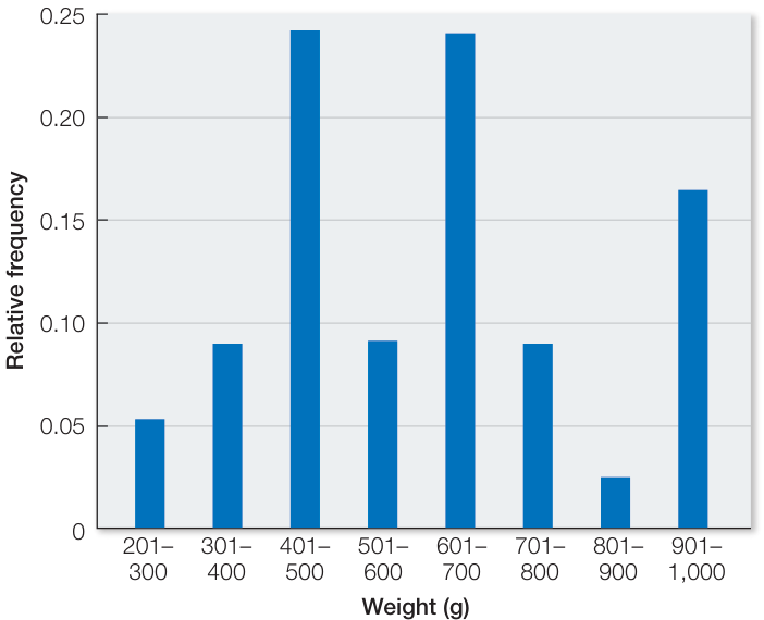
Figure B2 Histograms Depict Frequency Distributions of Quantitative Data This histogram shows the relative frequency of different weight classes of fish (Abramis brama).
Table B3 Poinsettia Colors
| Color | Frequency | Proportion |
|---|---|---|
| Red | 108 | 0.59 |
| Pink | 34 | 0.19 |
| White | 40 | 0.22 |
| Total | 182 | 1.0 |
Frequency distributions are also useful ways of summarizing categorical data. Table B3 shows a frequency distribution of the colors of 182 poinsettia plants (red, pink, or white) resulting from an experimental cross between two parent plants. Notice that, as with the fish example, the table is a much more compact way to present the data than a list of 182 color observations would be. For categorical data, the possible values of the variable are the categories themselves, and the frequencies are the number of observations in each category. We can visualize frequency distributions of categorical data like this by constructing a bar chart. The heights of the bars indicate the number of observations in each category (Figure B3). Another way to display the same data is in a pie chart, which shows the proportion of each category represented like pieces of a pie (Figure B4).
Sometimes we wish to compare two quantitative variables. For example, the researchers at Lake Laengelmavesi investigated the relationship between fish weight and length, from the data presented in Table B1. We can visualize this relationship using a scatter plot in which the weight and length of each fish is represented as a single point (Figure B5). These two variables have a positive relationship since the slope of a line drawn through the points is positive. As the length of a fish increases, its weight tends to increase in an approximately linear manner.
Tables and graphs are critical to interpreting and communicating data, and thus should be as self-contained and understandable as possible. Their content should be easily understood simply by looking at them. Axes, captions, and units should be clearly labeled, statistical terms should be defined, and appropriate groupings should be used when tabulating or graphing quantitative data.
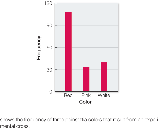
Figure B3 Bar Charts Compare Categorical Data This bar chart shows the frequency of three poinsettia colors that result from an experimental cross.
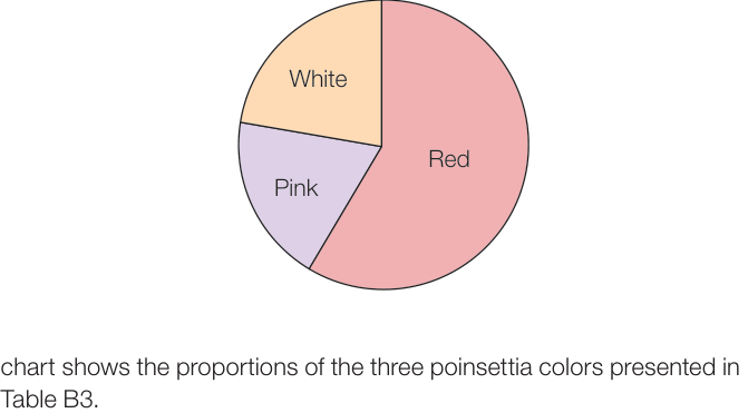
Figure B4 Pie Charts Show Proportions of Categories This pie chart shows the proportions of the three poinsettia colors presented in Table B3.
Step 4: Summarize the Data
A statistic is a numerical quantity calculated from data, whereas descriptive statistics are quantities that describe general patterns in data. Descriptive statistics allow us to make straightforward comparisons among different data sets and concisely communicate basic features of our data.
DESCRIBING CATEGORICAL DATA For categorical variables, we typically use proportions to describe our data. That is, we construct tables containing the proportions of observations in each category. For example, the third column in Table B3 provides the proportion of poinsettia plants in each color category, and the pie chart in Figure B4 provides a visual representation of those proportions.
DESCRIBING QUANTITATIVE DATA For quantitative data, we often start by calculating measures of center, quantities that roughly tell us where the center of our data lies. There are three commonly used measures of center:
- The mean, or average value, of our sample is simply the sum of all the values in the sample divided by the number of observations in our sample (Figure B6).
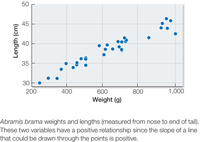
Figure B5 Scatter Plots Contrast Two Variables Scatter plot of Abramis brama weights and lengths (measured from nose to end of tail). These two variables have a positive relationship since the slope of a line that could be drawn through the points is positive.
- The median is the value at which there are equal numbers of smaller and larger observations.
- The mode is the most frequent value in the sample.
It is often just as important to quantify the variation in the data as it is to calculate its center. There are several statistics that tell us how much the values differ from one another. We call these measures of dispersion. The easiest one to understand and calculate is the range, which is simply the largest value in the sample minus the smallest value. The most commonly used measure of dispersion is the standard deviation, which calculates the extent to which the data are spread out from the mean. A deviation is the difference between an observation and the mean of the sample. The standard deviation is a measure of how far the average observation in the sample is from the sample mean. Two samples can have the same range, but very different standard deviations if observations in one are clustered closer to the mean than in the other. In Figure B7, for example, sample 1 has a smaller standard deviation () than does sample 2 (), even though the two samples have the same means and ranges.
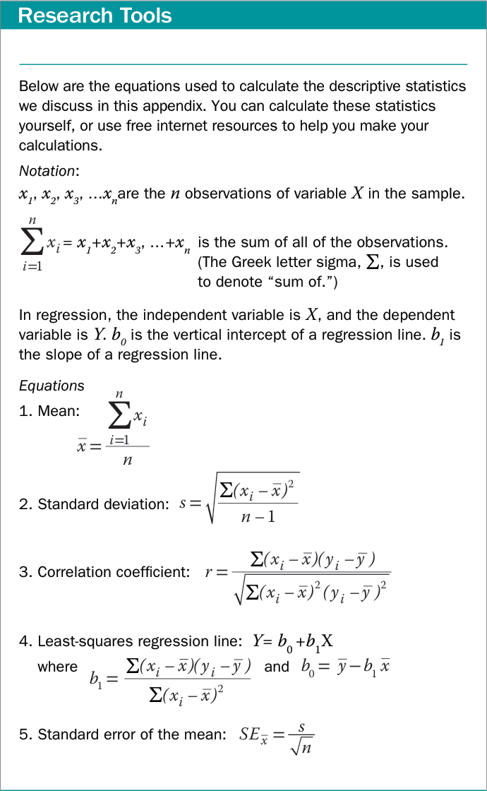
Figure B6 Descriptive Statistics for Quantitative Data
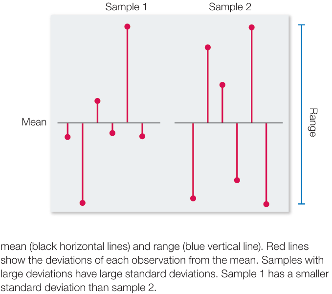
Figure B7 Measures of Dispersion Two samples with the same mean (black horizontal lines) and range (blue vertical line). Red lines show the deviations of each observation from the mean. Samples with large deviations have large standard deviations. Sample 1 has a smaller standard deviation than sample 2.
To demonstrate these descriptive statistics, let’s return to the Lake Laengelmavesi study (see the data in Table B1). The mean weight of the 34 fish (see equation 1 in Figure B6) is:
Since there is an even number of observations in the sample, then the median weight is the value halfway between the two middle values:
The mode of the sample is 500 g, which appears four times. The standard deviation (see equation 2 in Figure B6) is:
and the range is .
DESCRIBING THE RELATIONSHIP BETWEEN TWO QUANTITATIVE VARIABLES Biologists often are interested in understanding the relationship between two different quantitative variables: How does the height of an organism relate to its weight? How does air pollution relate to the prevalence of asthma? How does lichen abundance relate to levels of air pollution? Recall that scatter plots visually represent such relationships.
We can quantify the strength of the relationship between two quantitative variables using a single value called the Pearson product–moment correlation coefficient (see equation 3 in Figure B6).
This statistic ranges between and and tells us how closely the points in a scatter plot conform to a straight line. A negative correlation coefficient indicates that one variable decreases as the other increases; a positive correlation coefficient indicates that the two variables increase together; and a correlation coefficient of zero indicates that there is no linear relationship between the two variables (Figure B8).
One must always keep in mind that correlation does not mean causation. Two variables can be closely related without one causing the other. For example, the number of cavities in a child’s mouth correlates positively with the size of his or her feet. Clearly cavities do not enhance foot growth; nor does foot growth cause tooth decay. Instead the correlation exists because both quantities tend to increase with age.
Intuitively, the straight line that tracks the cluster of points on a scatter plot tells us something about the typical relationship between the two variables. Statisticians do not, however, simply eyeball the data and draw a line by hand. They often use a method called least-squares linear regression to fit a straight line to the data (see equation 4 in Figure B6). This method calculates the line that minimizes the overall vertical distances between the points in the scatter plot and the line itself. These distances are called residuals (Figure B9). Two parameters describe the regression line: (the vertical intercept of the line, or the expected value of variable when ), and (the slope of the line, or how much values of are expected to change with changes in values of ).
Step 5: Inferential Statistics
Data analysis often culminates with statistical inference—an attempt to draw general conclusions about the system under investigation—the larger population—from observations of a representative sample (see Figure B1). When we test a new medulloblastoma brain cancer drug on ten patients, we do not simply want to know the fate of those ten individuals; rather, we hope to predict the drug’s efficacy on the much larger population of all medulloblastoma patients.
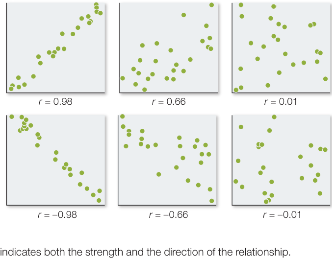
Figure B8 Correlation Coefficients The correlation coefficient ( ) indicates both the strength and the direction of the relationship.
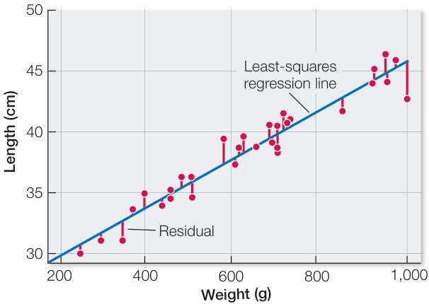
Figure B9 Linear Regression Estimates the Typical Relationship between Two Variables Least-squares linear regression line for Abramis brama weights and lengths (measured from nose to end of tail). The regression line (blue line) is given by the equation . It is the line that minimizes the sum of the squares of the residuals (red lines).
STATISTICAL HYPOTHESES Once we have collected our data, we want to evaluate whether or not they fit the predictions of our hypothesis. For example, we want to know whether or not cancer incidence is greater in our sample of smokers than in our sample of nonsmokers, whether or not clutch size increases with spider body weight in our sample of spiders, or whether or not growth of a sample of fertilized plants is greater than that of a sample of unfertilized plants.
Before making statistical inferences from data, we must translate our “whether or not” question into a pair of opposing statistical hypotheses. Often our “whether” hypothesis is difficult to translate because it does not make specific predictions such as how much greater the cancer incidence should be in smokers compared with nonsmokers, or how much clutch size will increase with body weight, or how big the growth advantage of fertilized plants will be. For this reason, scientists often evaluate the “whether” hypothesis indirectly by calculating the fit of the data to an opposing “or not” hypothesis that does make a specific prediction. This “or not” hypothesis is often called the null hypothesis (denoted ) because it proposes that there is no difference between sample means, or no correlation between variables in the sample, or no difference between our sample and an expected frequency distribution. The statistical alternative hypothesis (denoted ) is often our biological hypothesis: that there is a difference in means, or that there is a correlation between variables, or that the sample distribution does differ from the expected one. We base our conclusion about our biological hypothesis on the fit of our data to the null hypothesis because it is so difficult to calculate the fit to the many alternative hypotheses.
Suppose, for example, we would like to know whether or not a new vaccine is more effective than an existing vaccine at immunizing children against influenza. We have measured flu incidence in a group of children who received the new vaccine and want to compare it with flu incidence in a group of children who received the old vaccine. Our statistical hypotheses would be as follows:
: Flu incidence was the same in both groups of children.
: Flu incidence was different between the two groups of children.
In the next few sections we will discuss how we decide when to reject the null hypothesis in favor of the alternative hypothesis.
JUMPING TO THE WRONG CONCLUSIONS There are two ways that we can draw incorrect conclusions from a statistical test (Figure B10). We can reject the null hypothesis when it is actually true (Type I error), or we can accept the null hypothesis when it is actually false (Type II error). These kinds of errors are analogous to false positives and false negatives in medical testing, respectively. If we mistakenly reject the null hypothesis when it is actually true, then we falsely endorse the incorrect alternative hypothesis. If we mistakenly accept the null hypothesis when it is actually false, then we falsely reject the correct alternative hypothesis.
Fortunately, statisticians have developed statistical tests to minimize the chance of committing these kinds of errors and to increase our confidence in the reliability of our conclusions. The methods are based on calculating the probabilities of obtaining different possible data values. Although you may have heard or even used the word “probability” on multiple occasions, it is important that you understand its mathematical meaning. A probability is a numerical quantity that expresses the chance of making a particular observation. It ranges between 0 and 1; 0 means that the observation never occurs, and 1 that the observation always occurs. This makes sense only if there is an element of chance—that is, if alternative observations are possible. For example, in a coin flip, heads and tails are possible observations. Similarly, when we select an individual from a human population, we may select a female or a male, or when we select an Abramis brama from Lake Laengelmavesi, its length can take on any number of values.
Probability is at the core of statistics. To draw conclusions about the real world (the population) from our sample, we first calculate the probability of obtaining the data in our sample if the null hypothesis is true. We refer to this probability as the P-value of our test. Specifically, we ask “What is the probability of observing what we see or measure in our random sample from the total population if the null hypothesis is true?” If our sample is highly improbable under the null hypothesis, then we gain confidence in the alternative hypothesis.
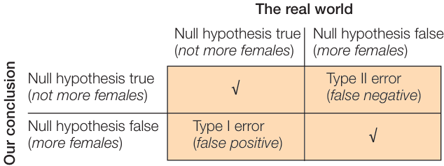
Figure B10 Two Types of Errors Possible outcomes of a statistical test. Statistical inference can result in correct and incorrect conclusions about the population of interest.
To take an example, suppose we would like to know whether there are equal numbers of females and males in a population of 10,000 students. To determine the makeup of the population, we choose 20 individuals at random and record their sex. Our null hypothesis is that the sex ratio in the population is 50:50, and our alternative hypothesis is that the sex ratio is not 50:50. Suppose that our sample contains 5 women and 15 men. The probability by chance alone of a sex ratio that skewed or more, if the sex ratio is really 50:50, turns out to be 0.02 (that is, 2%). (We will explain below how to arrive at this -value.)
What sense can we make of this result and its -value? We are justified in being skeptical that the population from which we drew the sample really has a 50:50 sex ratio. Yes, it’s possible to randomly choose 5 women and 15 men if the null hypothesis is true, but we would expect this outcome in only 2% of all samples of 20 students that we could take. Said another way, if we are wrong and the sex ratio is actually 50:50, we have made a Type I error, but the chance of doing that is only 2%. We will likely go ahead to reject the null hypothesis and instead conclude that the sex ratio is not 50:50 in the population of 10,000 students.
Now, suppose instead that our sample of 20 students contains 8 women and 12 men. Here (that is, 44%). What can we conclude from this result? We are much less certain about rejecting the null hypothesis that the sex ratio is 50:50. The -value means that 44% of samples would be this skewed, or more, if the sex ratio were 50:50.
With a result like this, we are tempted to conclude that the sex ratio indeed is 50:50, and it is a common practice to accept the null hypothesis when the -value is moderate. But this action might very well represent a Type II error (accepting a false hypothesis). Note that a probability of 44% of obtaining our result if the sex ratio is 50:50 is not very strong support for that specific null hypothesis. Other hypotheses, such as a hypothesis that the student population actually contains 40% women and 60% men (the observed proportions) fit the data even better than the null hypothesis of a 50:50 sex ratio.
For this reason, it is better to conclude simply that we cannot reject the null hypothesis when we obtain a moderate -value. How moderate does the -value have to be for us to conclude this? It has become conventional to use (5%) as a cutoff, and to label a result with as “significant” and one with as “not significant.” You should keep in mind, however, that is not some magic number that determines whether one or another hypothesis is absolutely “proved” or “falsified.”
What can we do to go further, with the example of for our sample sex ratio? If possible, we could obtain additional samples (for example, of 20 individuals) from the overall population, to gather more information on the underlying sex ratio. But this sort of replication of sampling may often be impossible or impractical. Fortunately, it may not matter in many cases, because what often is critical is to minimize the chance of making a Type I error of rejecting a true null hypothesis. Once again, think of a clinical trial of a new drug, using a sample of patients. If we obtain a very small -value—a very small chance of a Type I error—when we compare patients chosen at random to receive the drug with those receiving a placebo, then we gain confidence that the drug works. If the -value is relatively large, then we accept the null hypothesis that the drug is not effective, and we aren’t very concerned about a Type II error of accepting a false null hypothesis in this case. We are looking to see whether the drug has a strong beneficial effect. If it does not have a strong effect, we are not so interested in finding out whether its effect is exactly zero or just close to zero.
This agrees with our intuition. When choosing 20 people randomly from an evenly divided population, we would be surprised if almost all of them were female, but we would not be surprised at all if we ended up with a few more females than males (or a few more males than females). Exactly how many females do we need in our sample before we can confidently infer that they make up the majority of the population? And how confident are we when we reach that conclusion? Statistics allows us to answer these questions precisely.
STATISTICAL SIGNIFICANCE: AVOIDING FALSE POSITIVES
Whenever we test hypotheses, we calculate the probability just discussed, and refer to this value as the -value of our test. Specifically, the -value is the probability of getting data as extreme as our data (just by chance) if the null hypothesis is in fact true. In other words, it is the probability that chance alone would produce data that differ from the null hypothesis as much as our data differ from the null hypothesis. How we measure the fit of our data to the null hypothesis depends on the kind of data in our sample (categorical or quantitative) and the nature of the null hypothesis (assertions about proportions, single variables, multiple variables, differences between variables, correlations between variables, etc.).
For many statistical tests, -values can be calculated mathematically. One option is to quantify the extent to which the data depart from the null hypothesis and then use look-up tables (available in most statistics textbooks or on the internet) to find the probability that chance alone would produce a difference of that magnitude. Most scientists, however, find -values primarily by using statistical software rather than hand calculations combined with look-up tables. Regardless of the technology, the most important steps of the statistical analysis are still left to the researcher: constructing appropriate null and alternative hypotheses, choosing the correct statistical test, and drawing correct conclusions.
After we calculate a -value from our data, we have to decide whether it is small enough to conclude that our data are inconsistent with the null hypothesis. This is decided by comparing the -value to a threshold called the significance level, which is often chosen even before making any calculations. We reject the null hypothesis only when the -value is less than or equal to the significance level, denoted . This ensures that, if the null hypothesis is true, we have at most a probability of rejecting it when it is true. Therefore the lower the value of , the less likely you are to make a Type I error (see the lower left cell of Figure B10). The most commonly used significance level is , which limits the probability of a Type I error to 5%.
If our statistical test yields a -value that is less than our significance level , then we conclude that the effect described by our alternative hypothesis is statistically significant at the level and we reject the null hypothesis. If our -value is greater than , then we conclude that we are unable to reject the null hypothesis.
POWER: AVOIDING FALSE NEGATIVES The power of a statistical test is the probability that we will correctly reject the null hypothesis when it is false (see the lower right cell of Figure B10). Therefore the higher the power of the test, the less likely we are to make a Type II error (see the upper right cell of Figure B10). The power of a test can be calculated, and such calculations can be used to improve your methodology. Generally, there are several steps that can be taken to increase power and thereby avoid false negatives:
- Increase the value of . The lower the value of (our significance level), the harder it is to reject the null hypothesis, even if it is actually false.
- Increase the sample size. The more data one has, the more likely one is to find evidence against the null hypothesis, if it is actually false.
- Decrease variability in the sample. The more variation there is in the sample, the harder it is to discern a clear effect (the alternative hypothesis) when it actually exists.

Simulation B.6 Power of Statistical Tests
It is always a good idea to design your experiment to reduce any variability that may obscure the pattern you seek to detect. For example, it is possible that the chance of a child contracting influenza varies depending on whether he or she lives in a crowded (e.g., urban) environment or one that is less so (e.g., rural). To reduce variability, a scientist might choose to test a new influenza vaccine only on children from one environment or the other. After you have minimized such extraneous variation, you can use power calculations to choose the right combination of and sample size to reduce the risks of Type I and Type II errors to desirable levels.
There is a trade-off between Type I and Type II errors: as decreases, the risk of a Type I error decreases but the risk of a Type II error increases. As discussed above, scientists tend to be more concerned about Type I than Type II errors. However, there are many real-world scenarios in which it would be worse to make a Type II error than a Type I error. For example, suppose a new cold medication is being tested for dangerous (life-threatening) side effects. The null hypothesis is that there are no such side effects. A Type II error might lead regulatory agencies to approve a harmful medication that could cost human lives. In contrast, a Type I error would simply mean one less cold medication among the many that already line pharmacy shelves. In such cases, policymakers take steps to avoid a Type II error, even if, in doing so, they increase the risk of a Type I error.
STATISTICAL INFERENCE WITH QUANTITATIVE DATA Statistics that describe patterns in our samples are used to estimate properties of the larger population. Earlier we calculated the mean weight of a sample of Abramis brama in Lake Laengelmavesi, which provided us with an estimate of the mean weight of all the Abramis brama in the lake. But how close is our estimate to the true value in the larger population? Our estimate from the sample is unlikely to exactly equal the true population value. For example, our sample of Abramis brama may, by chance, have included an excess of large individuals. In this case, our sample would overestimate the true mean weight of fish in the population.
The standard error of a sample statistic (such as the mean) is a measure of how close it is likely to be to the true population value. The standard error of the mean, for example, provides an estimate of how far we might expect a sample mean to deviate from the true population mean. It is a function of how much individual observations vary within samples (the standard deviation) and the size of the sample (). Standard errors increase with the degree of variation within samples, and they decrease with the number of observations in a sample (because large samples provide better estimates about the underlying population than do small samples). For our sample of 34 Abramis brama, we would calculate the standard error of the mean using equation 5 in Figure B6:
The standard error of a statistic is related to the confidence interval—a range around the sample statistic that has a specified probability of including the true population value. The formula we use to calculate confidence intervals depends on the characteristics of the data, and the particular statistic. For many types of continuous data, the bounds of the 95% confidence interval of the mean can be calculated by taking the mean and adding and subtracting 1.96 times the standard error of the mean. Consider our sample of 34 Abramis brama, for example. We would say that the mean of 626 grams has a 95% confidence interval from 556.6 grams to 695.4 grams ( grams). If all our assumptions about our data have been met, we would expect the true population mean to fall in this confidence interval 95% of the time.
Researchers typically use graphs or tables to report sample statistics (such as the mean) as well as some measure of confidence in them (such as their standard error or a confidence interval). This book is full of examples. If you understand the concepts of sample statistics, standard errors, and confidence intervals, you can see for yourself the major patterns in the data, without waiting for the authors to tell you what they are. For example, if samples from two groups have 95% confidence intervals of the mean that do not overlap, then you can conclude that it is unlikely that the groups have the same true mean.

Simulation B.7 Standard Deviations, Standard Errors, and Confidence Intervals Simulation
Biologists conduct statistical tests to obtain more precise estimates of the probability of observing a given difference between samples if the null hypothesis that there is no difference in the populations is true. The appropriate test depends on the nature of the data and the experimental design. For example, we might want to calculate the probability that the mean weights of two different fish species in Lake Laengelmavesi, Abramis brama and Leusiscus idus, are the same. A simple method for comparing the means of two groups is the t-test, described in Figure B11. We looked earlier at data for Abramis brama; the researchers who collected these data also collected weights for six individuals of Leusiscus idus: 270, 270, 306, 540, 800, and 1,000 grams. We begin by stating our hypotheses and choosing a significance level:
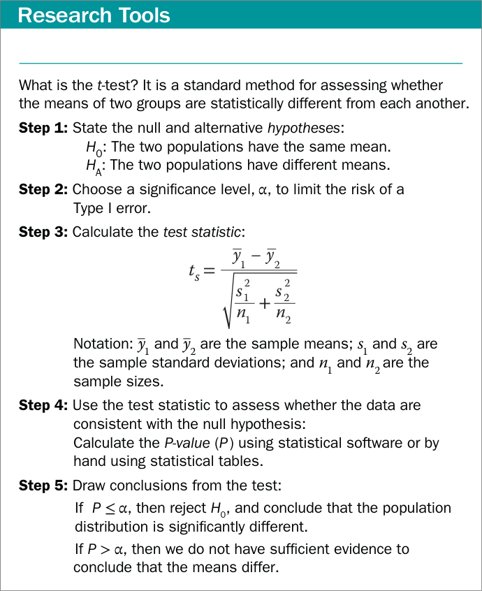
Figure B11 The t-test Figure B11 The t-test
: Abramis brama and Leusiscus idus have the same mean weight.
: Abramis brama and Leusiscus idus have different mean weights.
The test statistic is calculated using the means, standard deviations, and sizes of the two samples:
We can use statistical software or one of the free statistical sites on the internet to find that the P-value for this result is . Since is considerably greater than , we fail to reject the null hypothesis and conclude that our study does not provide evidence that the two species have different mean weights.
You may want to consult an introductory statistics textbook to learn more about confidence intervals, t-tests, and other basic statistical tests for quantitative data.
STATISTICAL INFERENCE WITH CATEGORICAL DATA With categorical data, we often wish to ask whether the frequencies of observations in different categories are consistent with a hypothesized frequency distribution. We can use a chi-square goodness-of-fit test to answer this question.
Figure B12 outlines the steps of a chi-square goodness-of-fit test. As an example, consider the data described in Table B3. Many plant species have simple Mendelian genetic systems in which parent plants produce progeny with three different colors of flowers in a ratio of 2:1:1. However, a botanist believes that these particular poinsettia plants have a different genetic system that does not produce a 2:1:1 ratio of red, pink, and white plants. A chi-square goodness-of-fit can be used to assess whether or not the data are consistent with this ratio, and thus whether or not this simple genetic explanation is valid. We start by stating our hypotheses and significance level:
: The progeny of this type of cross have the following probabilities of each flower color:
Figure B12 The Chi-Square Goodness-of-Fit Test
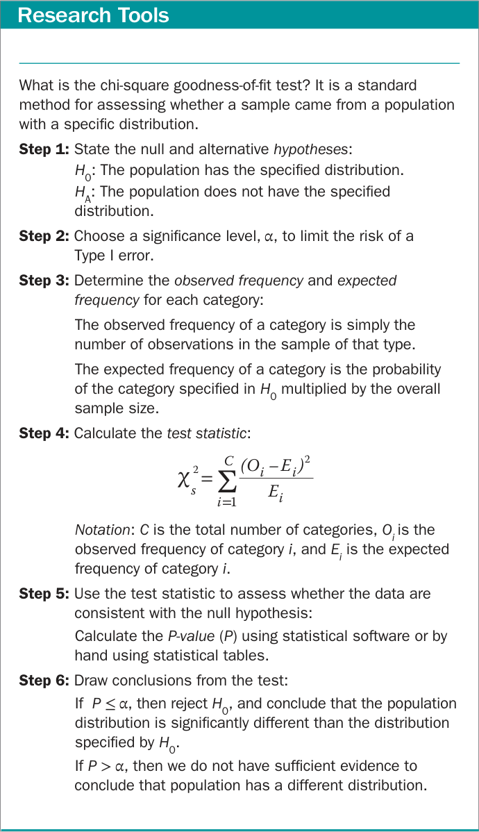
Figure B12 The Chi-Square Goodness-of-Fit Test
: At least one of the probabilities of is incorrect.
We next use the probabilities in and the sample size to calculate the expected frequencies:
| Red | Pink | White | |
|---|---|---|---|
| Observed | 108 | 34 | 40 |
| Expected |
Based on these quantities, we calculate the chi-square test statistic:
We find the -value for this result to be using statistical software. Since is less than , we reject the null hypothesis and conclude that the botanist is likely correct: the plant color patterns are not explained by the simple Mendelian genetic model under consideration.
This appendix is meant to provide only a brief introduction to the concepts of statistical analysis, with a few example tests. Figure B13 summarizes some of the commonly used statistical tests that you may encounter in biological studies.
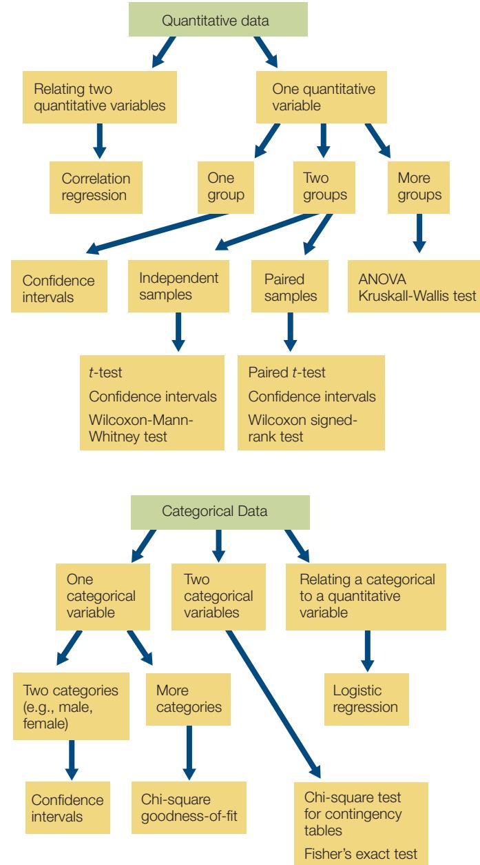
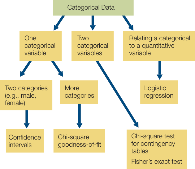
Figure B13 Some Common Methods of Statistical Inference This flowchart shows some of the commonly used methods of statistical inference for different combinations of data. Detailed descriptions of these methods can be found in most introductory biostatistics textbooks.