Chapter 52The Physical Environment and Biogeography of Life
© Merley Beaz/Alamy Stock Photo
Key Concepts
- 52.1 Ecology Is the Study of the Interrelationships among Organisms and the Environment
- 52.2 Global Climate Is a Fundamental Component of the Physical Environment
- 52.3 Topography, Vegetation, and Humans Modify the Physical Environment
- 52.4 Biogeography Is the Study of How Organisms Are Distributed on Earth
- 52.5 Geographic Area and Humans Affect Regional Species Diversity
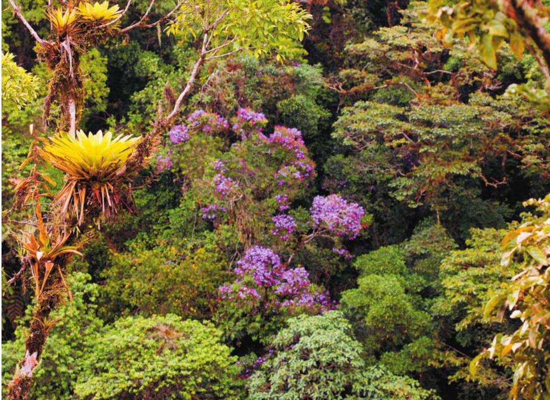
Amazonian forests, such as this, contain half of all the described species on Earth.
Investigating Life: The Largest Experiment on Earth
Most people know that there are many species on Earth, and that new species are being discovered every day, but not everyone knows that roughly half of all species worldwide reside in one place: the tropical rainforests of the Amazon Basin. The statistics are staggering: an estimated 390 billion trees representing 16,000 species grow in Amazonia, one in five bird species globally resides there, and one-fifth of all fresh water falls on its slopes and valleys. The Amazon Basin is by far the largest watershed on Earth, with thousands of tributaries leading to the Amazon River and then out to sea. To date, 2,200 freshwater fish species have been described, which is more than all the fish species in the Atlantic Ocean.
It is reasonable to assume, then, that when the Amazon Basin is threatened by human activities, so, too, is global biodiversity. By far, the main destructive force is deforestation, which began about 50 years ago. As roads pushed their way into Amazonia’s forests, more rainforest was logged and converted to agriculture and settlements. It is estimated that nearly 20% of the Amazon Basin has been clear-cut. Because soil fertility is generally poor in tropical rainforests, the cleared land is often useful only for a decade or less, resulting in abandonment and new cycles of deforestation and fragmentation.
How does habitat fragmentation affect the species living in the Amazon Basin? Fragmentation makes habitats smaller, and it isolates populations. Deforestation forces species to sustain themselves in a smaller area or move to more suitable areas. In the late 1970s, some ecologists asked a deceptively simple question about Amazon deforestation: What is the minimum area needed to maintain species diversity within a rainforest fragment? They wanted to know whether the species remaining in the forest fragments could maintain themselves there, whether the sizes of the forest fragments mattered to this maintenance, and whether species would venture from one fragment to another. These ecologists conducted a large and long-running experiment in the Amazon forests near Manaus, Brazil. As you will see in Key Concept 52.5, the size of the fragments and the ability of species to move across the deforested landscape are key to maintaining the extraordinary diversity left in the Amazon Basin.
QA How do geographic area and isolation affect the biogeography of life on Earth? (Find the answer on page 1194.)
Ecology Is the Study of the Interrelationships among Organisms and the Environment
Learning Objectives
- 52.1.1 Distinguish between ecology and environmentalism, and give examples of each.
- 52.1.2 Explain the levels of organization in ecology, and be able to distinguish them from one another based on spatial scale.
- 52.1.3 Describe the research methods used by ecologists, and identify how and why ecological studies might differ from studies in other scientific fields.
Whether you notice ants collecting crumbs on a sidewalk or watch a video of polar bears hunting on sea ice, you are studying ecology. From simple experiences such as these, most people know that organisms on Earth are interconnected with one another and with their environment. Ecology is the exploration of these interconnections and is most simply defined as the study of the interrelationships among organisms and the physical environment. Ecologists study these interactions at different scales and with different methods, but they all agree that ecology is a scientific endeavor, first and foremost.
“Ecology” is sometimes equated with “environmentalism,” but the two terms are different. Ecology is a science that generates knowledge about interactions in the natural world. Environmentalism is the use of ecological knowledge, along with economics, ethics, and many other considerations, to inform both personal decisions and public policy related to stewardship of the natural world. So while an ecologist might study the number of bluefin tuna in the world’s oceans, the environmentalist would focus on the social, economic, and political capital needed to enforce a sustainable harvest or, alternatively, to ban bluefin tuna fishing altogether.
Ecology is a relatively new branch of the biological sciences; in fact, it did not have a formal name until 150 years ago when Ernst Haeckel, a German biologist, constructed the new word “ecology,” from the Greek root oikos, meaning “household.”
Modern ecology has a more “use-inspired” focus
Although it was recognized in Darwin’s day that humans could affect the natural world, and that human populations were undergoing unprecedented growth, for the most part early ecologists believed they were studying pristine systems largely untouched by human activities. Today most ecologists have a much greater awareness of ways in which humans shape the natural world, be it in the form of global climate change, the introduction of novel species to new locations, or the logging of Earth’s tropical forests. Because of the dominant role that humans play in almost every ecological system on Earth, a “use-inspired” motivation often shapes ecologists’ research and teaching. They understand that scientific knowledge of ecology greatly improves our ability to grow food for ourselves reliably and sustainably, to manage pests and diseases safely and effectively, and to deal with natural disasters such as floods and fires. The greater our understanding of ecological connections, the more likely it is that we can accomplish these things without causing a cascade of unanticipated consequences for ourselves and the other life on Earth.
Ecology is studied at many levels of organization
Ecology is studied at many levels of organization, from molecules to the entire globe. Some ecologists work at the level of genes to understand how individuals might adapt to a changing environment, while other researchers seek to understand how temperature might modify nutrient cycling at the ecosystem level. The work of ecologists focuses on many scales or levels of organization: individuals, populations, communities, ecosystems, landscapes, or the global biosphere (Figure 52.1).
As prior chapters have conveyed, a population is a group of individuals of the same species within a given area that have the potential to interbreed and interact with one another. For example, the individual sea stars in Figure 52.1 make up a population at this particular rocky shore location. The sea star population in turn interacts with other species, including its prey, sessile mussels, and its competitors, whelks and other sea star species. These species form a community, which is an assemblage of interacting species living together at the same place and time.
Ecological studies often encompass both the living, or biotic, and the nonliving, or abiotic, components of the environment. The biotic components of an organism’s environment are other organisms, so ecology includes the study of interactions within and among species. The abiotic components of an organism’s environment are the myriad physical and chemical characteristics of the system. For example, in the rocky shore community, tides are a key abiotic factor because they limit where sea stars can feed on mussels and compete with whelks.
The term ecosystem is often used when describing a community of organisms in which their physical environment is explicitly taken into account. Ecosystem ecology particularly focuses on the movement of energy and nutrients through a group of organisms. The movement of energy and nutrients, as well as organisms, can affect higher levels of organization, including landscapes, geographic areas that include multiple ecosystems (sometimes referred to as meta-ecosystems). Ultimately, meta-ecosystems are linked to one another at larger geographic scales to form the biosphere, consisting of all living organisms on Earth plus their respective environments.
Answering ecological questions requires observations, experiments, and models
Just as in other fields in biology, ecologists use a mixture of observations, experiments, and models to test ecological theories (see Key Concept 1.3). Ecologists are unique, though, in using a wide range of venues and scales in their experiments, including short laboratory experiments, long-term field manipulations, and even decades-long ecosystem-wide experiments, such as the Biological Dynamics of Forest Fragments Project described in Key Concept 52.5. However, at large spatial scales or over long periods of time, well-replicated and controlled experiments are usually not possible. For example, when studying the ecological effects of climate change on a particular species, ecologists might have to combine observations of the temperature range of that species with short-term experiments on the effects of warming on the species’ distribution and then use models to project how distributions could change with continued warming. Often this type of research requires multiple techniques and collaborative efforts to be successful.
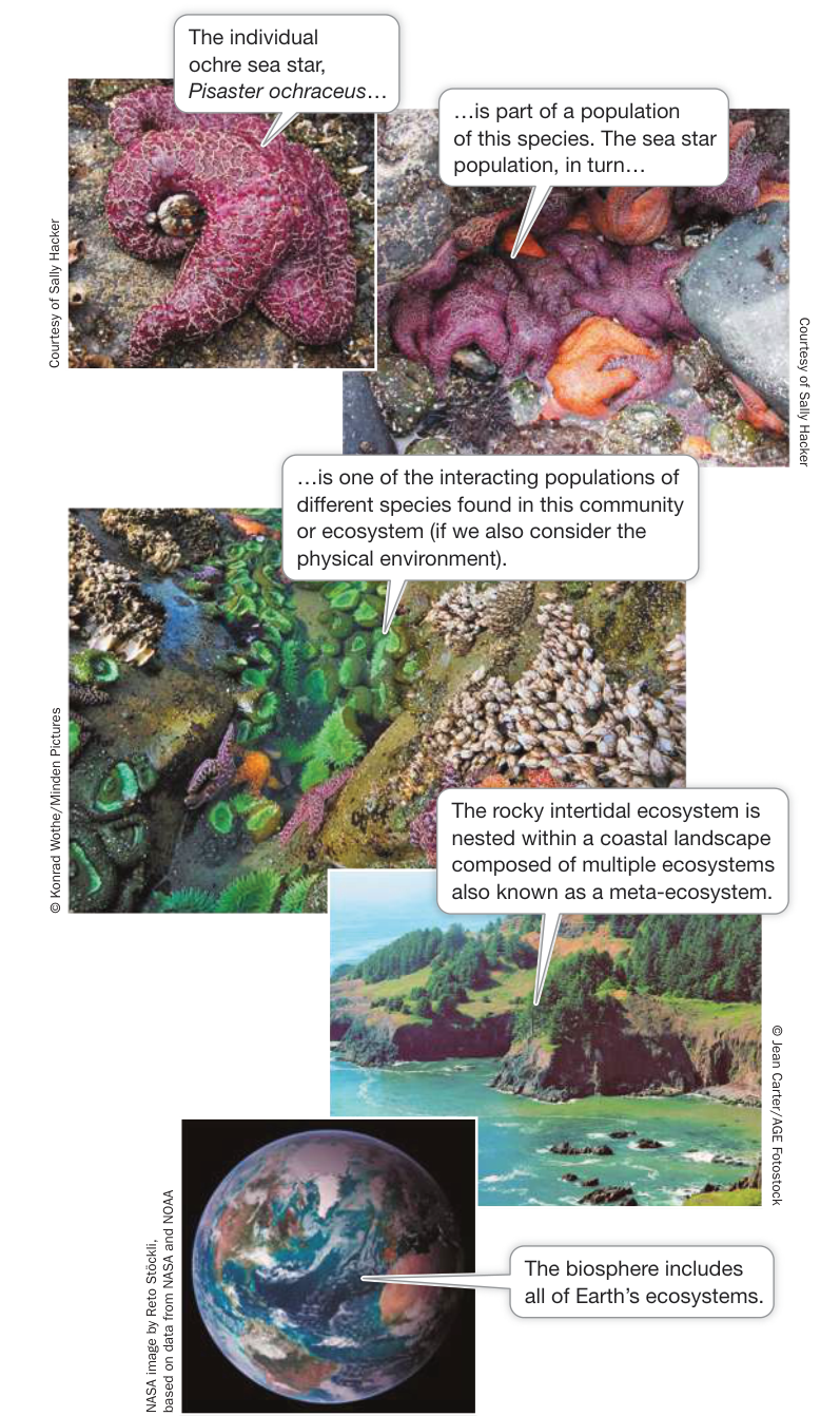
Figure 52.1 Scale Is Important to Ecological Systems These photos from the Oregon coast of the United States illustrate how ecological systems can be studied at multiple scales, from the individual to the biosphere.
Recap and Assess
Ecology is the scientific study of the interrelationships among organisms and the environment. Ecology is studied at multiple levels of organization, from individuals to the biosphere. Ecologists use a mixture of observations, experiments, and models to test ecological theories.
- Compare how an ecologist versus an environmentalist might approach an environmental problem.
- Using observations, experiments, and models at different levels of organization, describe how you might test the hypothesis that the widespread death of the ochre sea star (Pisaster ochraceus) (shown in Figure 52.1) is the result of a disease.
We will begin our study of ecology in the spirit of the discipline in Haeckel’s time, focusing on variations in the distribution and abundance of organisms worldwide and the factors that determine these patterns. Our first step will be to examine attributes of the physical environment, which is the most basic determinant for where organisms can live. We’ll begin with climate.
Global Climate Is a Fundamental Component of the Physical Environment
Learning Objectives
- 52.2.1 Compare weather and climate, and give examples of both.
- 52.2.2 Given that Earth is a sphere, has an atmosphere, and rotates around its axis, explain the latitudinal variation in temperature, precipitation, and prevailing winds.
- 52.2.3 Relate Earth’s prevailing wind patterns to ocean currents, and explain how ocean currents affect climate.
- 52.2.4 Connect the tilt of Earth’s axis and its orbit to the existence of seasons on Earth, and explain why the Northern and Southern Hemispheres have opposite seasonal patterns.
The terms “weather” and “climate” both refer to atmospheric conditions—temperature, humidity, precipitation, and wind direction and velocity—but they consider different time scales. Weather is the short-term state of atmospheric conditions at a particular place and time, whereas climate refers to the average atmospheric conditions, and the extent of their variation, at a particular place over a longer time (years to millennia). Climate is what you expect given past conditions; weather is what you get on any one day. For example, a warming climate will cause glaciers to melt over decades or centuries (see Figure 1.17), whereas a single large snowstorm is unlikely to slow that retreat. In addition, the responses of organisms to weather are usually short-term—seeking shelter from a sudden rainstorm, for example, or shivering to keep warm when the temperature drops. Climate, by contrast, acts as a sort of filter for organisms, ultimately determining their distribution and abundance. If organisms cannot tolerate the climate of a particular place, they will not be found there. Here we consider the processes that create climate patterns.
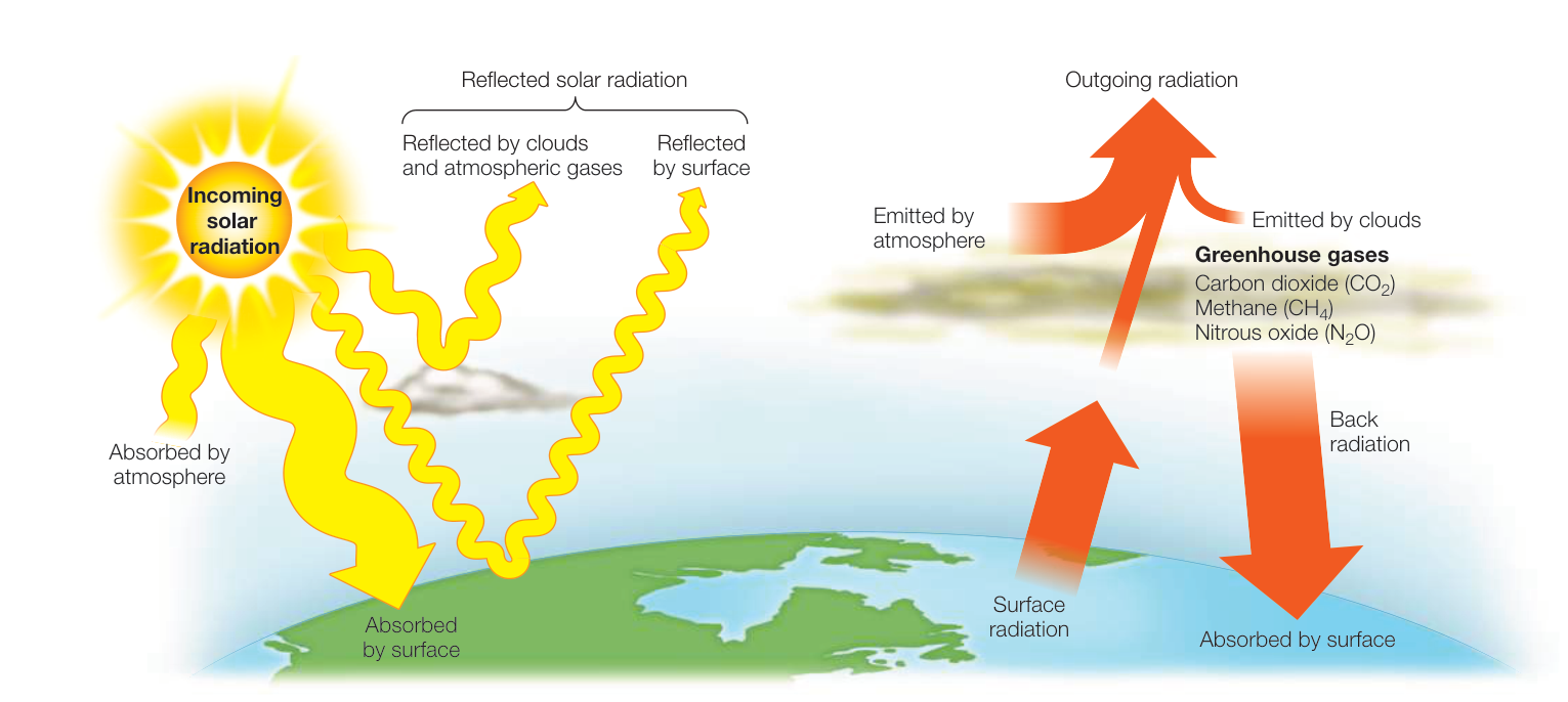
Figure 52.2 Radiant Energy Warms the Planet Solar energy input (yellow arrows) is absorbed by Earth’s atmosphere and surface. Much of this energy is radiated from Earth’s surface in the form of heat (orange arrows). Of that absorbed at the surface, most is prevented from escaping back into space by greenhouse gases in the atmosphere. The widths of the arrows are roughly proportional to the sizes of the energy fluxes. (After K. E. Trenberth et al. 2009. Bull Am Meteorol Soc 90: 311–323; Lindsey, R. 2009. Climate and Earth’s energy budget. Earth Observatory, EOS Project Science Office, NASA Goddard Space Flight Center. Greenbelt, MD.) Q: What effect do greenhouse gases have on Earth’s energy balance?
Solar radiation drives global climate patterns
The energy that drives global climate patterns ultimately originates from the Sun. Of the solar radiation that hits Earth, about 30% is reflected back to space by clouds, atmospheric gases, and Earth’s surface (Figure 52.2). The rest is absorbed either by the atmosphere (20%) or the surface of Earth (50%). The atmosphere, a thin layer of gases surrounding Earth composed of nitrogen gas ( , 78%), oxygen ( , 21%), argon (0.9%), carbon dioxide ( , 0.037%), and traces of hydrogen, helium, ozone, methane (), and many other gases, moderates Earth’s surface temperatures by trapping heat energy. If Earth had no atmosphere, its average surface temperature would be about , rather than its actual . Carbon dioxide, methane, nitrous oxide (), water vapor, and certain other gases in the atmosphere are known as greenhouse gases because they allow sunlight into Earth’s atmosphere but trap heat radiating back out toward space (see Figure 52.2).
The amount of radiation received on Earth varies with latitude and with the seasons. These differences are driven by some well-known characteristics of Earth: it is a sphere that orbits the Sun, it spins on a tilted axis, and it has both land and water. As you will see, it is the combination of these factors that determines the climate we experience on Earth.
Earth is a sphere, creating latitudinal variation in global temperature and precipitation
Because Earth is a sphere, the intensity of solar radiation hitting its surface varies with latitude. This latitudinal variation in solar energy depends primarily on the angle of the Sun’s rays striking
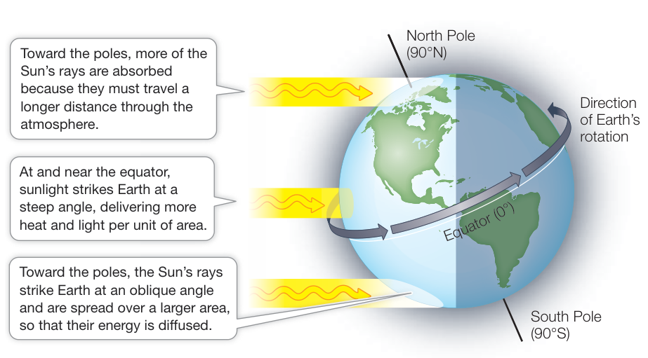
Figure 52.3 Solar Energy Input Varies with Latitude The angle of incoming sunlight affects the intensity of solar energy that reaches a given unit of Earth’s surface. (After C. D. Ahrens. 2005. Essentials of Meteorology: An Invitation to the Atmosphere. Brooks/Cole, Cengage Learning: USA.)
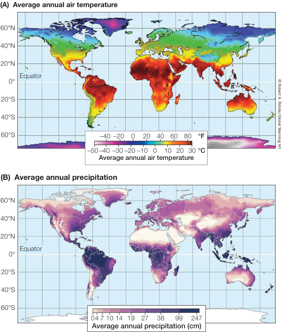
Figure 52.4 Global Temperature and Precipitation Vary with Latitude Average annual air temperature (A) and precipitation (B) vary with Earth’s latitude but can be modified by topography (i.e., Earth’s shape and surface features) (see Figure 52.9). (A, after Berkeley Earth. 2016. Land and Ocean Baseline Comparison Map. http://www.berkeleyearth.org/; B, courtesy of the Nelson Institute Center for Sustainability and the Global Environment [SAGE], through their “Atlas of the Biosphere,” https://nelson.wisc.edu/sage/data-and-models/atlas/. University of Wisconsin-Madison.)
Earth. At high latitudes (i.e., areas toward the North and South Poles), incoming solar energy is distributed over a larger area (and thus is less intense) than at the equator, where sunlight strikes the surface perpendicularly (Figure 52.3). Moreover, when the Sun’s radiation comes in at an angle, it must pass through more of Earth’s atmosphere, resulting in more of its energy being absorbed or reflected before reaching Earth’s surface. Differences in solar energy input explain why the average global temperature varies with latitude, with warmer temperatures at the equator and colder temperatures at the poles (Figure 52.4A). The average air temperature over the course of a year decreases about 0.76 degrees Celsius for every degree of latitude (~110 km) at sea level.
In addition to there being a latitudinal variation in temperature, the Northern Hemisphere is slightly warmer (by ~2 degrees Celsius) and more variable in temperature (by a range of ~7 degrees
Celsius) than the Southern Hemisphere (see Figure 52.4A). Although the reasons for this difference are uncertain, one hypothesis is that because land heats up the air above it more than does the ocean (which absorbs more heat), the greater proportion of land to ocean in the Northern Hemisphere creates warmer air temperatures than those in the Southern Hemisphere. This is particularly true in summer, when the temperature difference is at its greatest. In light of global warming, it is worth noting that temperatures are increasing faster in the Northern Hemisphere than in the Southern Hemisphere.
Besides controlling temperature, solar energy input also determines atmospheric circulation and associated precipitation patterns. As you saw earlier, air in the region surrounding the equator receives the greatest input of solar energy. When a parcel of air is warmed, it expands, becomes less dense, and rises (see Figure 52.5A). As it rises, however, it starts to cool at higher elevations. Cool air cannot hold as much water vapor as warm air, so the expanding, cooling air releases moisture in the form of precipitation. This is particularly evident in the tropics, where there is abundant rainfall year-round (Figure 52.4B). Eventually the rising air at the equator reaches the boundary between the troposphere, the atmospheric layer above Earth’s surface, and the stratosphere, the next layer up. The stratosphere is warmer than the troposphere at this boundary, causing the tropical air to stop rising and eventually move either north or south as newly warmed air rises to replace it (Figure 52.5A). Eventually this air starts to cool as it exchanges heat with the atmosphere and meets colder air traveling from higher latitudes. When this cool, dry air, which lost its moisture as it rose over the equator, reaches latitudes of about 30°N and 30°S, it begins to sink under high atmospheric pressure, making the climate at these latitudes dry (Figure 52.5B). Earth’s great deserts—including the Sahara of Africa, the Gobi of China, and the deserts of Australia and the North American Southwest—are located at these latitudes (see Figure 52.5B).
While some of the descending air flows back toward the equator, some of it flows toward the poles, setting up another atmospheric cell of air circulation at higher latitudes. At about 60° latitude, air rises again due to its warming at Earth’s surface (see Figure 52.5B). As this air rises, it cools and releases precipitation, creating wet climate conditions at temperate latitudes. Eventually this air reaches the stratosphere and moves north or south. The cold, dry air traveling at higher latitudes eventually reaches the cold polar region, where it descends. Despite the amount of snow and ice at the poles, high latitudes at or near 90° actually receive little precipitation and can be thought of as “polar deserts” (see Figure 52.5B).
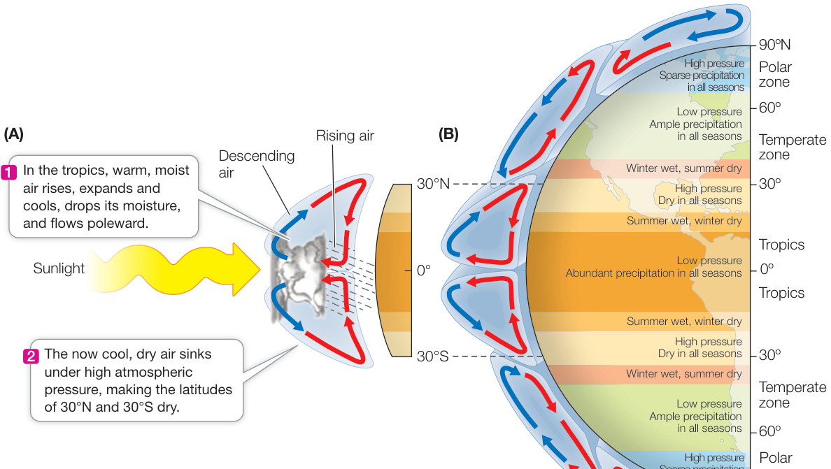
Figure 52.5 Air Circulation in Earth’s Atmosphere Drives Climate (A) Solar energy drives patterns of atmospheric circulation. (B) The differential heating of Earth’s surface by solar radiation gives rise to atmospheric circulation cells, which influence atmospheric pressure, air temperatures, and precipitation worldwide. (After C. D. Ahrens. 2005. Essentials of Meteorology: An Invitation to the Atmosphere. Brooks/Cole, Cengage Learning: USA.)
Earth spins on an axis, producing prevailing winds and ocean currents
You have seen that Earth’s spherical shape creates predictable patterns of temperature and precipitation, but Earth’s rotation, which moves east to west, is responsible for generating global wind and ocean currents. Because Earth is a sphere, the velocity of its rotation around its axis is fastest at the equator, where its diameter is greatest, and is slowest close to the poles. This difference creates the Coriolis effect, which is the deflection of air or water as a result of differences in Earth’s rotational speed at different latitudes. For example, air traveling toward the equator (driven by the circulation patterns described above and in Figure 52.5) moves at a slower speed than that of the planet beneath it and is thus deflected to the west. Conversely, air traveling toward either pole is moving faster than that of the surface beneath it and is deflected to the east. This interaction of Earth’s rotation and north-south air mass movement sets up a pattern of circulating surface air referred to as prevailing winds (Figure 52.6). Prevailing winds blow from east to west in the tropics (the trade winds); from west to east in mid-latitudes (the westerlies); and from east to west again above 60°N or 60°S latitude (the easterlies).
How, then, are the circulation patterns of ocean currents generated? Ocean currents are driven by prevailing winds, which move water by means of frictional drag. The trade winds, for example, cause currents to converge at the equator and move westward until they encounter a continent (Figure 52.7). At that point, the strong Equatorial Countercurrent brings some of the water back eastward. The remaining water divides, some moving northward and some southward along continental shores.
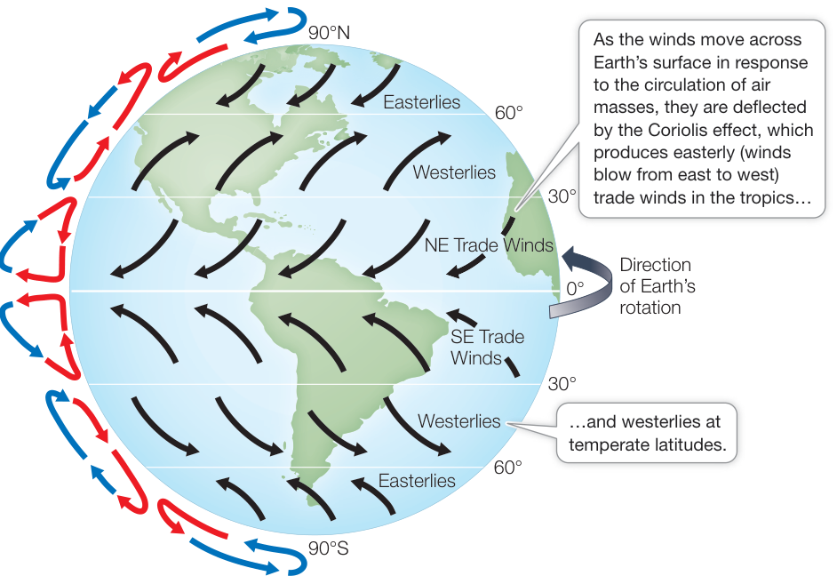
Figure 52.6 Prevailing Winds Created by Earth’s Rotation and Atmospheric Circulation The deflection of air as a result of differences in Earth’s rotational speed at different latitudes (also known as the Coriolis effect) coupled with atmospheric circulation of air masses combine to create a global pattern of prevailing surface winds across the planet.
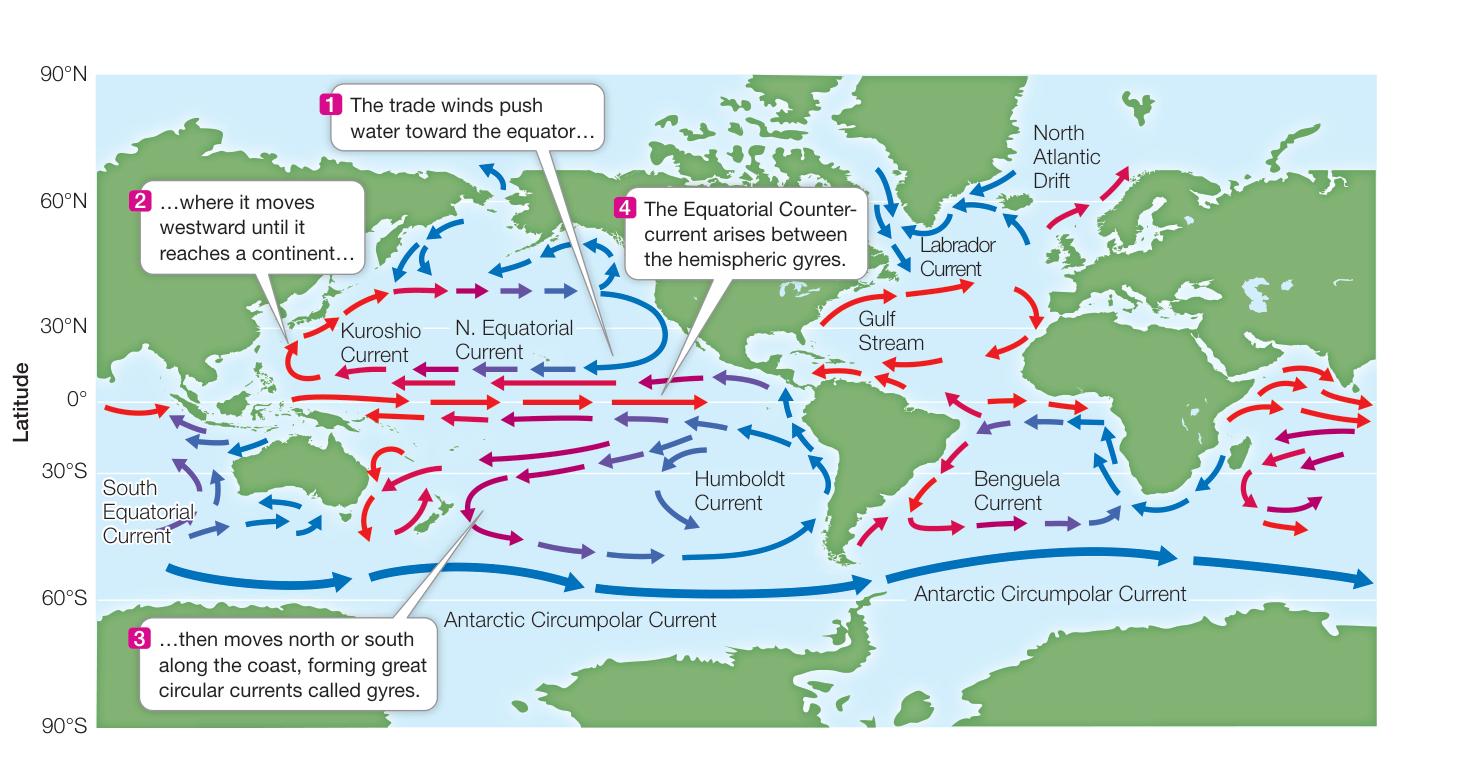
Figure 52.7 Oceanic Circulation Created by Winds and Continents The surface currents of the ocean are driven by the prevailing winds (see Figure 52.6), Earth’s rotation, and the placement of the continents. Red arrows indicate warm surface water, and blue arrows indicate cold surface water.
These patterns of water movement set up rotating circulation patterns called gyres (Greek gyros, “spiral”), which rotate clockwise in the Northern Hemisphere and counterclockwise in the Southern Hemisphere.
Because ocean currents transport heat, they have a tremendous effect on Earth’s climates. The poleward movement of warm water from the tropics transfers large amounts of heat to high latitudes. The Gulf Stream, for example, carries warm water from the tropical Atlantic Ocean (including the Gulf of Mexico) north across the Atlantic to northern Europe, making Europe’s climate considerably milder than that of some corresponding latitudes in North America. Similarly, currents flowing toward the equator from high latitudes bring cool, wet winters to some western coastal regions that are otherwise warm and dry.
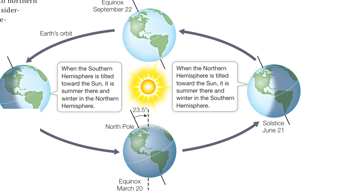
Figure 52.8 Seasonal Change Is the Result of the Tilt of Earth’s Axis and Its Orbit Because Earth’s axis of rotation is tilted, orientation relative to the Sun changes over the course of a year as the planet orbits the Sun. The resulting variation in solar radiation creates seasonal climate variation. (After C. D. Ahrens. 2005. Essentials of Meteorology: An Invitation to the Atmosphere. Brooks/Cole, Cengage Learning: USA.)
The tilt of Earth’s axis and its orbit result in seasons
The tilt of Earth’s axis, coupled with Earth’s orbit around the Sun, is responsible for seasonal changes in climate. Earth’s axis is tilted at an angle of 23.5 degrees, changing the amount of sunlight a particular region receives over the course of a year as Earth orbits the Sun (Figure 52.8). This tilt causes seasonal variation in temperature and day length. Higher latitudes experience greater seasonal variation than lower latitudes do. Around the equator, day length and seasonal temperatures change only slightly over the course of the year, although there are seasonal shifts in precipitation patterns.
Recap and Assess
Climate and weather both refer to atmospheric conditions, but climate represents conditions over years whereas weather represents conditions over a span of days. Earth is a sphere, has an atmosphere, and rotates around its axis, which creates latitudinal variation in solar radiation, temperature and precipitation, and prevailing winds and ocean currents. Earth’s tilt and orbit around the Sun result in the seasons.
- Does a month of extremely hot weather tell us that Earth’s climate is warming? Explain your answer.
- Refer to Figure 52.3. Why does solar energy input into Earth’s atmosphere vary with latitude? What are the consequences for global climate?
- Refer to Figures 52.6 and 52.7. If you were sailing, using wind power only, from the east coast of North America to Europe across the Atlantic Ocean, describe the best route given winds and currents.
- Explain why Earth’s Northern and Southern Hemispheres have opposite seasons.
We have considered large, global patterns in climate, but we know that the physical environment can vary within certain regions or even locally. Just travel across a large mountain range and you can experience lush forests on one side and bone-dry deserts on the other. We will turn next to what controls smaller, more regional and local variation in the physical environment, both on land and in water.
Topography, Vegetation, and Humans Modify the Physical Environment
Topography, Vegetation, and Humans Modify the Physical Environment
Learning Objectives
- 52.3.1 Explain and compare the causes and effects of rain shadows and temperature inversions.
- 52.3.2 Describe how ocean-floor topography creates variable marine environments.
- 52.3.3 Compare and contrast the effects of vegetation on temperature and precipitation at local and regional scales.
- 52.3.4 Describe and contrast ways in which agriculture and urbanization may transform local and regional climates.
Three main factors can modify the pattern of global climate, determining regional and local variation in climate and other aspects of the physical environment: (1) Earth’s topography, (2) vegetation, and more recently, (3) the effects of humans.
Earth’s topography affects the local and regional physical environment
Earth’s topography, meaning its shape and surface features, has been formed over geological time and provides the basis for much of the variation in local and regional physical conditions. Here we consider how topography modifies the physical environment with respect to land, oceans, rivers, and lakes.
LAND The topography of land plays a large role in the regional and local physical environment, including climate. Mountains create elevational gradients in temperature, precipitation, and sunlight. For example, mountains show progressively colder temperatures and greater precipitation at higher elevations, creating different environmental conditions over relatively short distances. When a mountain range occurs adjacent to an ocean, a rain shadow is often created, whereby one side of the mountain has a wet climate and the other side has a dry climate (Figure 52.9A). Rain shadows occur when winds deliver moist air evaporated from the ocean to the windward side of the mountain, where the air rises, cools, and releases rain or snow. On the leeward side of the mountain (that is, opposite from the direction of the winds), the now-dry air descends, warms, and produces arid conditions. The High Desert, on the leeward side of the Cascade Range in the Pacific Northwest of the United States, is one such area.
Other topographic features, such as canyons and valleys, also modify local climate in significant ways. Valleys can experience temperature inversions, extremes in temperature that produce morning fog and intense afternoon heat. Temperature inversions occur when the valley concentrates heat from solar radiation during the day. As that heat rises, it forms an inversion layer that traps cold, dense, and moisture-laden air that descends into the valley overnight and produces fog (Figure 52.9B).
OCEANS Beneath the oceans, which make up 70% of Earth’s surface, dramatic differences in topography influence the marine environment. If you could drain the oceans, you would notice major differences in topography, ranging from the Hawaiian island Mauna Loa, the tallest “mountain” on Earth at 9,170 meters high from base to peak, to the Mariana Trench, the deepest “valley” at 10,994 meters deep. Variations in water depth affect light penetration, water temperature, water pressure, and water movement (i.e., waves and tides). These physical discontinuities create distinct zones that are identified principally by their physical conditions and the characteristic biota they contain, similar to biomes on land (see Key Concept 52.4). The depth of an ocean basin varies from the shoreline to the relatively shallow continental shelf and to the deepest part of the ocean, sometimes known as the abyssal plain (Figure 52.9C). Water depth affects how much light is available to sustain the photosynthetic organisms that form the base of the marine food chain. In both marine and freshwater environments, roughly 90% of all aquatic life is found in the photic zone, the layer of water reached by enough sunlight to support photosynthesis.
Other zones that vary in environmental conditions include the coastal zone, which extends from the shoreline to the edge of the continental shelf, and the ocean zone, which extends beyond the coastal zone (see Figure 52.9C). The coastal zone is diverse and highly productive, supporting high densities of pelagic, or floating, plankton and fishes. On the benthos or bottom of the ocean, the coastal zone has a variety of living and nonliving habitats such as rocky reefs, soft sediment flats, coral reefs, and kelp beds. The portion of the benthic coastal zone lying between the high and low tide levels is the intertidal zone, where tidal movements create conditions of highly variable light and temperature, alternately exposing organisms to air and water. Intertidal zones can occur on the open coast as sandy or rocky beaches, or in more protected bays as estuaries. Estuaries form where rivers meet the sea, creating variability in salinity, sediment, and light conditions.
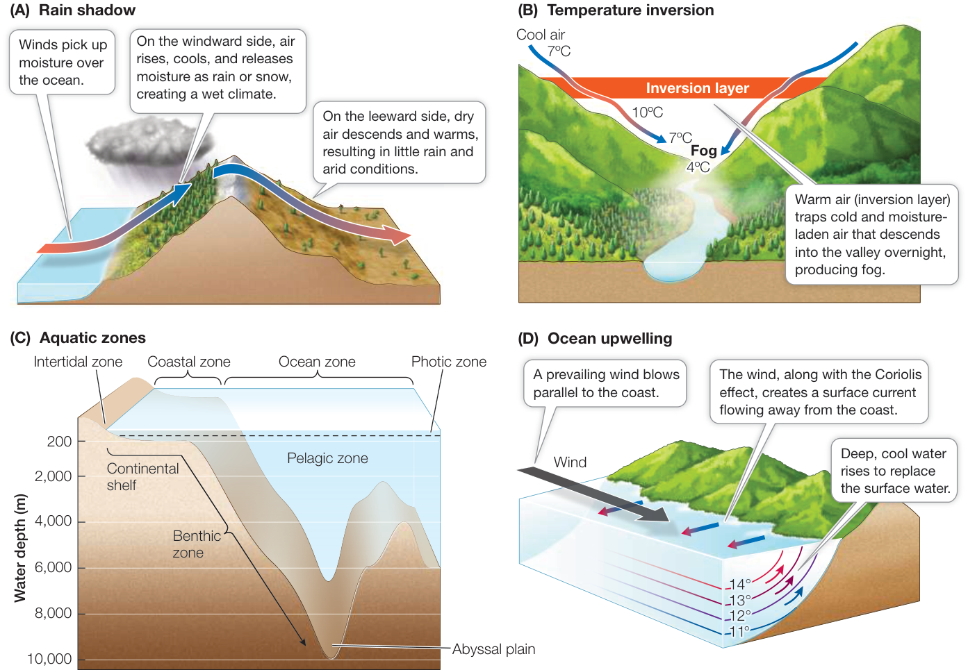
Figure 52.9 Effects of Earth’s Topography on the Physical Environment Earth’s topography can affect both land and oceans. Mountains and valleys create rain shadows (A) and temperature inversions (B). Ocean topography affects water depth, which creates aquatic zones that vary in light, temperature, and water pressure (C), and along with wind, produces ocean upwelling (D). (B after M. Schroeder and C. Buck. 1970. Fire Weather: A Guide for Application of Meteorological Information to Forest Fire Control Operations, p. 29. USDA Forest Service, Agriculture Handbook 360. D after C. D. Ahrens. 2005. Essentials of Meteorology: An Invitation to the Atmosphere. Brooks/Cole, Cengage Learning: USA.) Q: What kind of weather conditions would you expect to produce temperature inversions? How about ocean upwelling?
In some coastal zones, where the continental shelf drops off steeply and prevailing winds are parallel to the coastline, upwelling can affect ocean and climate conditions. Upwelling is a process in which offshore winds in combination with the Coriolis effect push warmer surface waters away from the shore, allowing deeper, colder, and nutrient-rich bottom water to rise to the surface (Figure 52.9D). Upwelling affects local and regional climate on the coast by creating cooler and moister conditions. In addition, upwelled waters support high rates of primary production by phytoplankton, which in turn support dense consumer populations. Most of the world’s great fisheries are concentrated in upwelling zones.
As we move away from the coastline, most of the ocean’s physical environment is made up of vast amounts of water that is, with the exception of the photic zone (which can extend to 200 meters in some regions), mostly dark, cold, and under tremendous pressure from the weight of the water above. Little photosynthesis can take place, and many of the organisms inhabiting these regions subsist on decaying organic matter that sinks down from the photic zone. Deep-ocean trenches and rift valleys support hydrothermal vent ecosystems sustained by chemoautotrophic prokaryotes that can metabolize the nutrients without the aid of sunlight (see Key Concept 24.3).
RIVERS AND LAKES In contrast to the vast oceans, freshwater lakes and rivers make up less than 3% of Earth’s surface, but they are home to about 10% of all aquatic species. Earth’s topography influences freshwater environments just as it does marine environments—through the depth of the water—but it also influences the degree and direction of movement of fresh water. A river is water that flows downhill from its point of origin (the source) over the land surface as a result of gravity until it reaches either the ocean or a depression in Earth’s surface, where it forms a lake or pond. The headwaters (those close to the source) tend to be cool, fast-flowing, and well oxygenated. As a river flows downstream, it widens, it slows down, it warms, and sediment accumulates, reducing light penetration and oxygen levels.
The Amazon River, mentioned in the chapter opening, offers a dramatic example of river dynamics. The Amazon is one of the longest rivers on Earth, at approximately 7,000 km. Eventually this source water reaches the Atlantic Ocean, where discharge is the largest of any river on Earth—the Amazon’s mouth is 240 km wide and is referred to as “the River Sea.”
Vegetation affects the local and regional physical environment, especially climate
Earth’s climate would be very different without the influence of organisms, including humans. Organisms can “engineer” the environment in multiple ways that affect the surrounding climate and physical conditions. The most obvious influence comes from vegetation, especially forests, which can have large effects on temperature and precipitation at local and even regional scales. For example, measurements of energy exchange in tropical forests that have been converted to pastureland show that forests make the climate cooler and moister (Figure 52.10). While forests absorb heat by reflecting less sunlight (reflection of solar radiation is known as the albedo effect) and decrease convective heat loss by acting as a wind screen, this is more than balanced by the cooling effect produced by evapotranspiration: the evaporative transfer of heat and water from the surfaces of plants into the atmosphere, which reduces air temperature and increases moisture. When forests are cut and replaced by vegetation such as grasses, the albedo effect and convective heat loss intensify while evapotranspiration decreases, causing overall air temperatures to rise and precipitation to decrease, creating more arid conditions. The climate changes associated with deforestation have been seen in the Amazon Basin, where massive forest clearing makes way for cattle ranching.
Oceans have their own “forests”—coastal areas dominated by seaweeds such as giant kelps or sea grasses that create calmer waters, promote sedimentation, and provide habitat for fishes and invertebrates. In warmer coastal waters, corals generate complex reef structures that support ecosystems rivaling rainforests in diversity. In Chapter 56 you will learn more about organisms that engineer their environment, but for now let’s turn to the final topic in this key concept: the effects of humans on climate and the physical environment.
Humans have transformed their physical environment, including urban climate
It is estimated that humans have transformed more than 50% of Earth’s land surface, replacing it with infrastructure and agriculture needed to support our burgeoning population. You have already seen how the conversion of forestland to pastureland can change regional climate, and in Chapter 56 you will learn more about how humans have changed global climate through the burning of fossil fuels. Structures such as dams, bridges, and nuclear power plants can dramatically transform rivers and lakes. Urban areas, in particular, modify not only the immediate physical environment but also the surrounding climate. A survey of 60 U.S. cities in 2014 showed that urban summer temperatures were on average 1.5 degrees Celsius hotter than rural summer temperatures, with the top 10 cities having an average urban–rural temperature differential of 5 degrees Celsius. The cause of this so-called urban heat island effect is simple: concrete, asphalt, and even the dark roofs of buildings absorb heat from solar radiation and radiate that heat in the evening hours (Figure 52.11). Cities also produce more heat through the burning of fossil fuels from cars, factories, and buildings. Parks can serve to cool the surrounding air through the evapotranspiration of trees and other vegetation. In addition, the temperature differential between cities and the surrounding countryside can create “country breezes,” air movement generated as rising warm air from the city is replaced by cold surface air from surrounding rural areas.
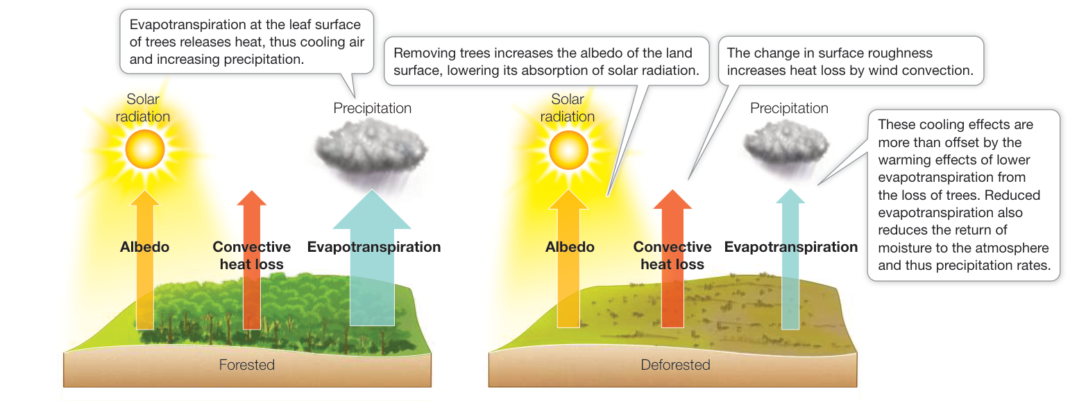
Figure 52.10 Deforestation Can Affect Climate Evapotranspiration by trees reduces air temperatures and increases precipitation. When land is deforested and the trees are gone, the cooling effects of the albedo (reflection of solar radiation) and of convective heat loss are not enough to outweigh the warming effects of reduced evapotranspiration. The widths of the arrows are roughly proportional to the sizes of the fluxes. (After J. A. Foley, et al. 2003. Front Ecol Environ 1: 38–44.)
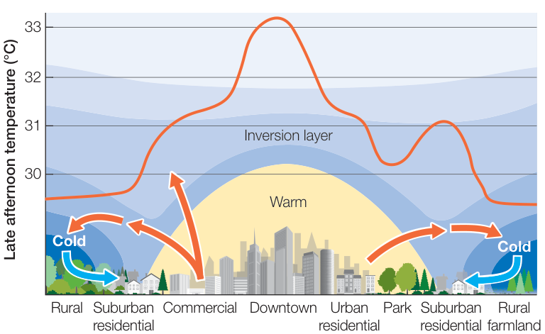
Figure 52.11 Cities Can Create Heat Islands and Country Breezes As this hypothetical urban heat island profile shows, cities and suburbs typically have higher temperatures than rural, park, or agricultural areas. Country breezes form when warm air from cities and suburbs is replaced by cool air from rural areas. (After D. Reidel. 2004. In Climate Change Impacts and Adaptation: A Canadian Perspective, D. S. Lemmen and F. J. Warren (Eds.), p. 157. Ottawa, ON: Climate Change Impacts and Adaptation Program, Natural Resources Canada; and H. E. Landsberg. 1970. Science 170: 1265–1274.)
Recap and Assess
Earth’s topography is responsible for rain shadows and temperature inversions, producing variation in temperature and precipitation. In the oceans, topographical variability produces differences in water depth, which affects light penetration, water temperature, water pressure, and water movement. Vegetation, especially forests, affects climate through the process of evapotranspiration. Cities can create their own climate; cities are on average hotter than rural areas.
- What are some of the major ways that Earth’s topography affects land and ocean physical conditions?
- Why are cities warmer than rural areas, and what are country breezes? How and why could the temperature in a city be changed with the establishment of a large forested park?
With an understanding of how Earth’s physical environment, including climate, is determined at a variety of spatial scales, we will turn next to biogeography: how the physical environment and other geographic and historical processes determine the global distribution of organisms on Earth.
Biogeography Is the Study of How Organisms Are Distributed on Earth
Learning Objectives
- 52.4.1 Describe the principle characteristics of each major biome, including climate, latitude and/or continent(s), and representative plants and animals.
- 52.4.2 Use the observations and insights of Alfred Russel Wallace to explain how biogeography might influence the distribution of plants and animals.
- 52.4.3 Compare and contrast the hypotheses posed for latitudinal patterns of species diversity, including species diversification rate, species diversification time, and productivity.
Biogeography is the scientific study of the distribution and diversity of organisms on Earth. “Distribution” is simply where organisms are found. “Diversity,” however, has multiple facets, which we will explore in more detail in Chapter 56, but for now you can think of it simply as the number and composition of species or higher taxa. For centuries, the processes that control these biogeographic patterns have puzzled naturalists. Why do species vary in their distributions around Earth, and what controls this variability?
Patterns of biogeography are interconnected across a hierarchy of spatial and temporal scales
The patterns of biogeography play out over global, regional, landscape, and local spatial scales (Figure 52.12). Spatial scales are interconnected in a hierarchical way, with patterns at one scale setting the conditions for patterns at other scales.
At the global scale, species are isolated from one another by continents or oceans, and for long periods of time. Thus the rates of three processes—speciation, extinction, and dispersal—help determine differences in biogeography across the globe (see Figure 52.12A). At the regional scale, large-scale climate conditions are relatively uniform and species are limited by their ability to disperse, or move between locations (see Figure 52.12B). All the species that are limited to a region are part of the regional species pool (also called gamma diversity). At the landscape scale, there are multiple community types—for example, lakes, rivers, forests, and prairies—arranged in a spatially heterogeneous way across the region (see Figure 52.12C). The change in the number of species from one community to another across the landscape is known as beta diversity. Finally, the local scale (also called alpha diversity) typically encompasses a single community—a group of species assembled together as the result of the physical environment, biotic interactions with other species, and the regional species pool (see Figure 52.12D).
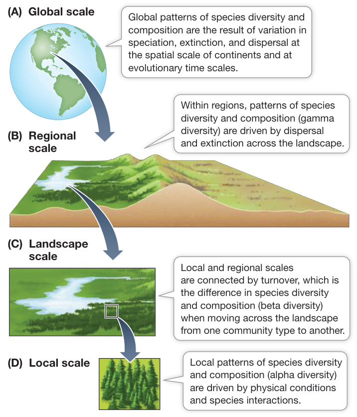
Figure 52.12 Biogeography Depends on Interconnected Spatial and Temporal Scales The arrows represent the relationship between, and processes important to, species diversity and composition at (A) global, (B) regional, (C) landscape, and (D) local scales. Q: At what scales is the regional species pool important to species diversity and composition?
In the remainder of this chapter we will consider the distributional and diversity patterns of organisms at global and regional biogeographic scales. Chapter 55 will consider the causes and consequences of diversity at community and local scales.
Terrestrial biomes reflect global patterns of temperature and precipitation
Biomes are groupings of ecologically similar organisms shaped by the environment in which they are found. The classification of biomes is most often and easily applied to terrestrial systems. Ecologists classify terrestrial biomes principally by the growth forms of their dominant plants, which reflect the evolution of those plants under annual patterns of temperature and precipitation.
The same classic types of biomes may be widely separated, occurring on different continents, depending in large part on the presence of suitable climatic conditions (Figure 52.13). For example, the desert biome occurs in such distant locations as Arizona in the North American Southwest and the Namib Desert in Africa;
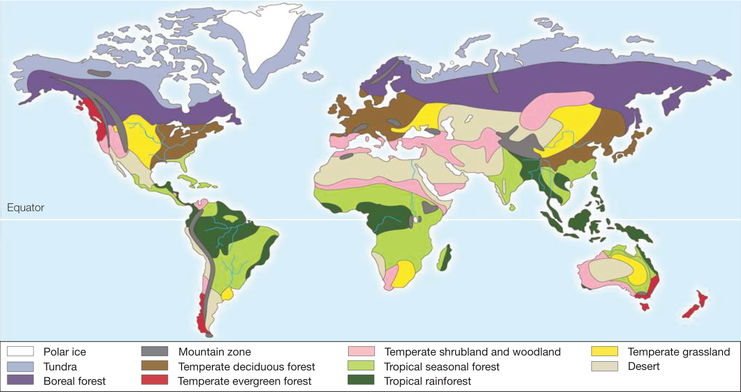
Figure 52.13 Global Distribution of Terrestrial Biomes The distribution of terrestrial biomes is determined primarily by annual patterns of temperature and precipitation.
Q: Does the Northern or Southern Hemisphere have a greater number of biome types? What do you think might determine this difference?
both locations are extremely dry and dominated by succulent plants such as cacti and by drought-tolerant shrubs and grasses. Why use plants as a way of classifying biomes? Because plants are immobile, they must adapt to environmental conditions in order to be successful over long periods of time. Thus the growth forms of plants strongly reflect their environment in ways that can be compared around the world. Furthermore, by providing three-dimensional structure, by modifying physical conditions near the ground, and by providing food, dominant plants strongly influence the organisms living there.
Connect the Concepts Key Concept 37.1 describes how plants growing in a particular type of environment (e.g., the desert) may display similar growth forms (e.g., succulence).
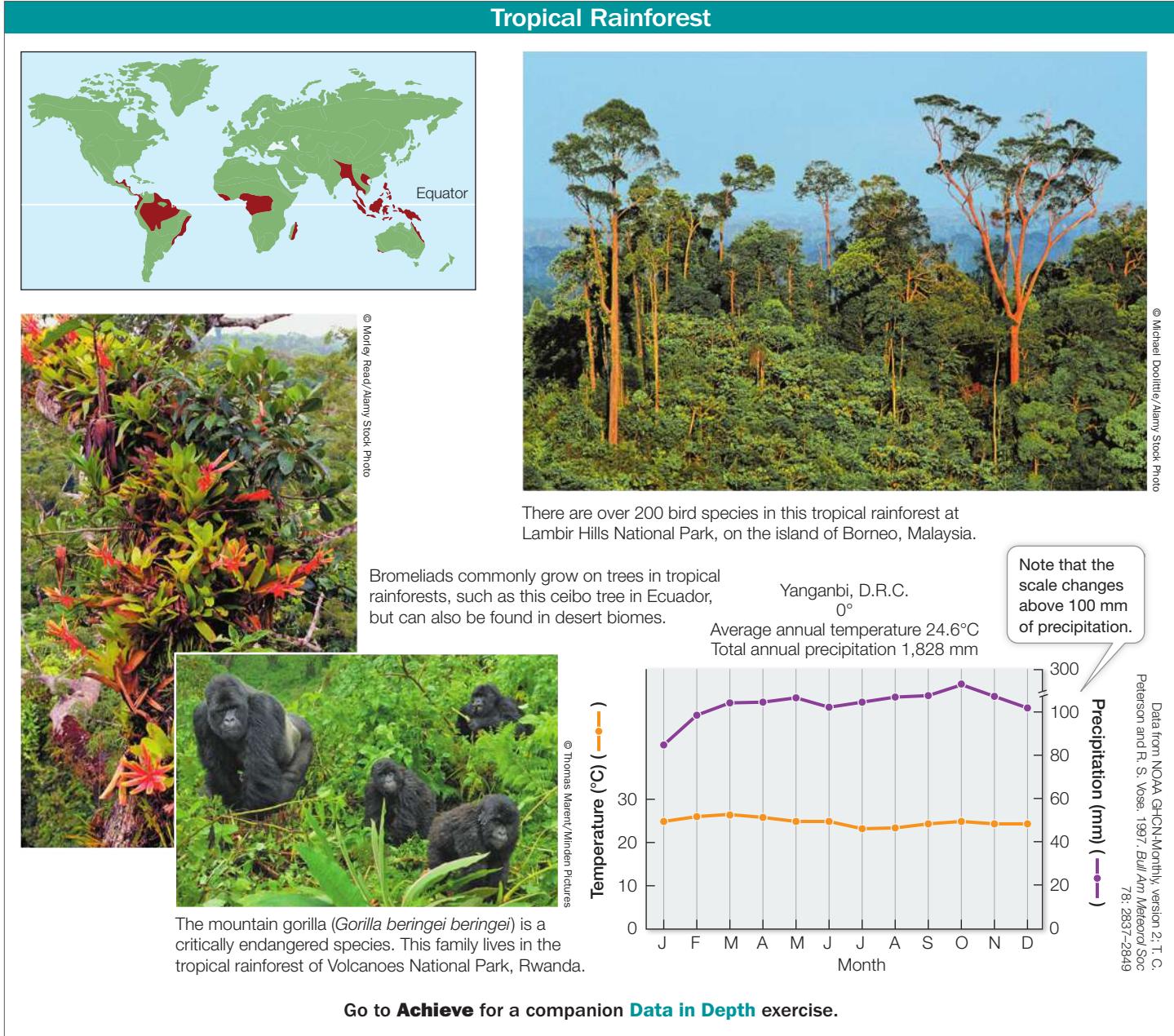
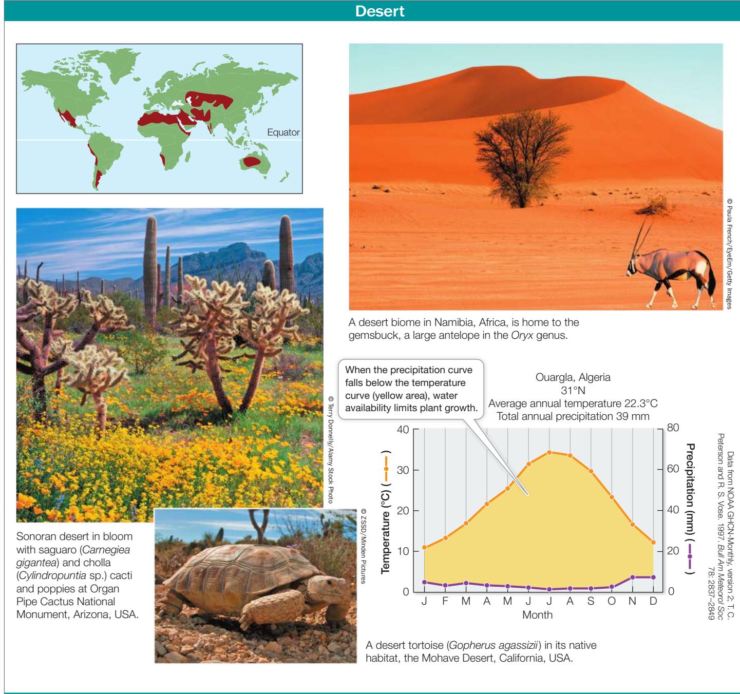
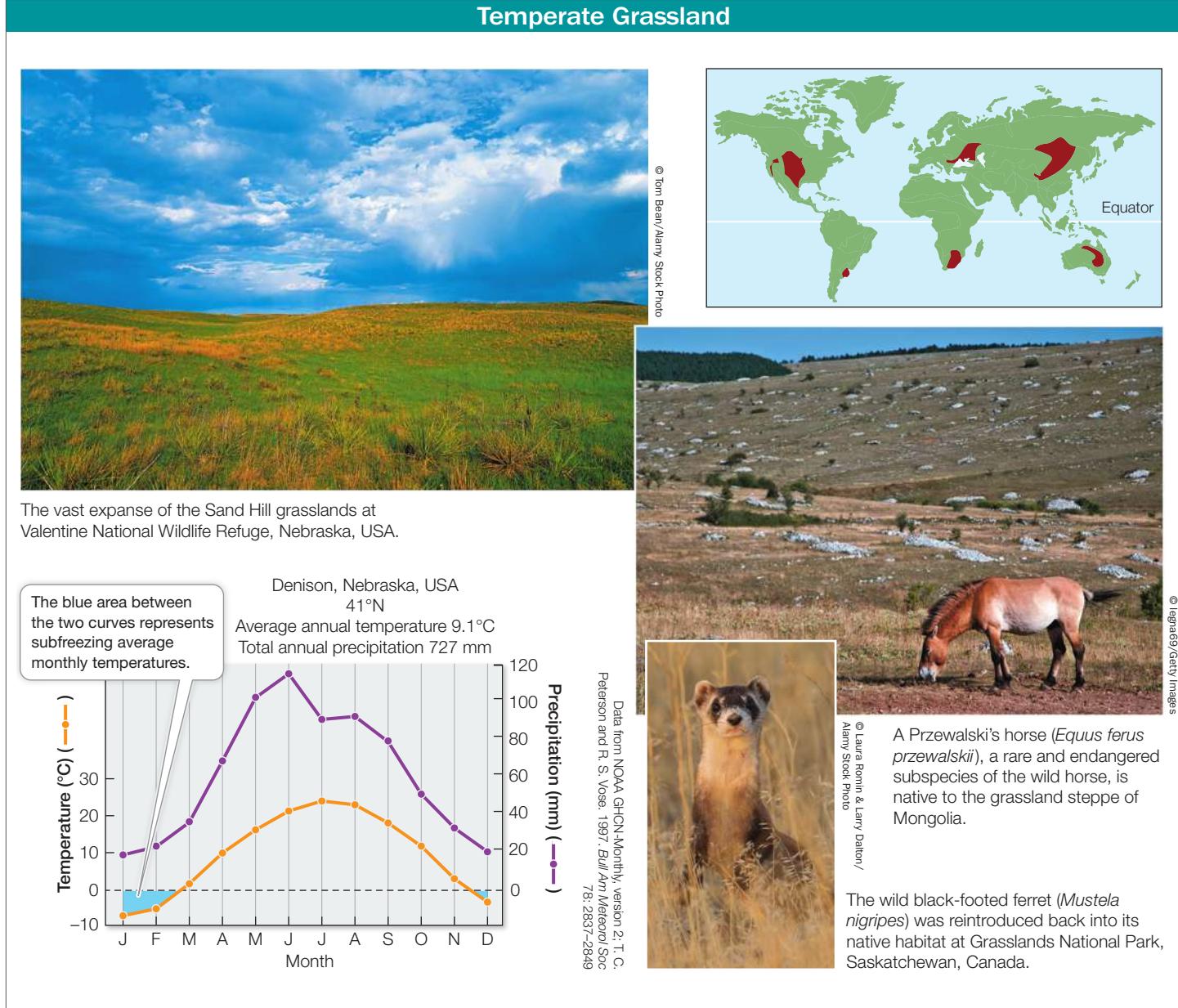
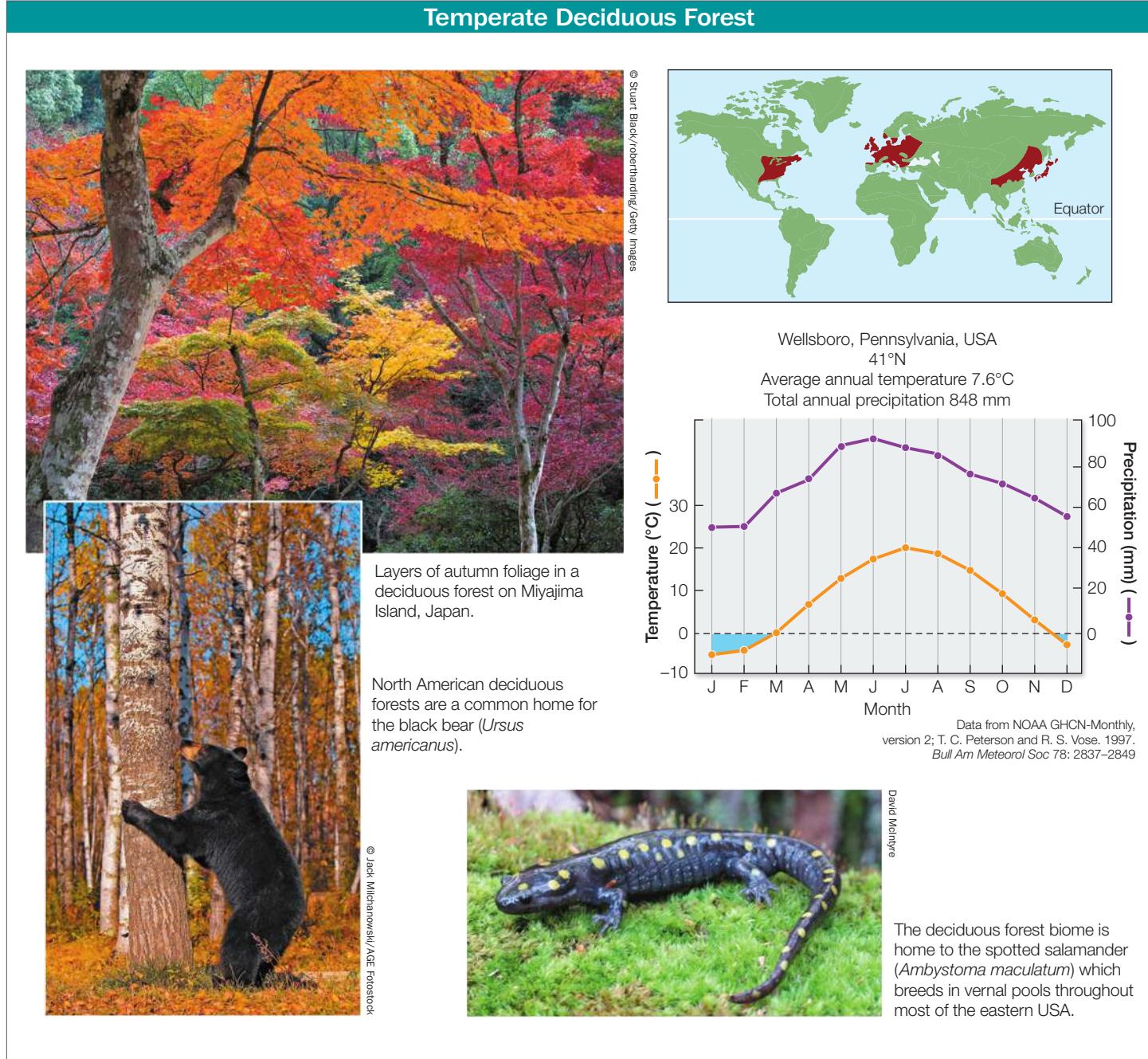
In the following pages we briefly describe seven terrestrial biomes (a subset of those shown in Figure 52.13). For each, a plot of the seasonal patterns of temperature and precipitation—known as a Walter climate diagram—is included. Devised by the German biogeographers Heinrich Walter and Helmut Lieth, this graphic technique plots temperature and precipitation data in a simple way that visualizes a “growing season”—those months when average temperatures are above freezing (0°C) and when average precipitation is sufficient for plant growth. Walter climate diagrams are predicated on the “rule of thumb” that plant growth requires temperatures above 0°C and at least 2 mm of precipitation for each 1-degree-Celsius rise in temperature. They have two y-axis scales, one for temperature and one for precipitation; these axes align 0 mm of precipitation with 0°C of temperature. The x axis shows 12 months, with the summer solstice placed in the center of the axis.
TROPICAL RAINFOREST The tropical rainforest biome is found in equatorial regions where rainfall and temperatures are high year-round. With no season unsuitable for growth, it is the most productive and species-rich of all biomes. In some areas, there are up to 500 species of trees per square kilometer. Although historically these forests covered 12% of Earth’s surface, and are now reduced through deforestation, they are home to more than half of all known species. These forests are home to many epiphytes—plants that grow on other plants, deriving their nutrients and moisture from air and water rather than soil.
Tropical rainforests provide humans with a range of products, including fruits, nuts, medicines, fuel, pulp, and furniture wood. Rainforests, however, are currently being cut down or converted to agriculture at a rate of almost 1% per year. In some cases, rainforests are recovering, but the soils are often nutrient-poor, hindering regrowth.
DESERT The desert biome is concentrated in two belts, centered around 30°N and 30°S latitude (where warm, dry air sinks under high atmospheric pressure; see Figures 52.4 and 52.5). The driest of these regions, where rains rarely fall, are far from the oceans, as in the center of Australia and the middle of the Sahara in Africa.
Desert plants have several structural and physiological adaptations that help them conserve water, as described in Key Concept 37.1. Small desert animals are inactive during the hottest part of the day, remaining in underground burrows. Desert mammals have physiological adaptations for conserving water, including a reduced number of sweat glands and kidneys that produce highly concentrated urine. Many desert animals require no water beyond what they can extract from the carbohydrates in their food.
Humans have used deserts for livestock grazing and agriculture for centuries. Deserts can be irrigated from deep wells or distant mountains, but such efforts typically fail as a result of salinization, the buildup of salts from the evaporation of irrigation water.
TEMPERATE GRASSLAND Temperate grasslands are found in many parts of the world, all of which are relatively dry for much of the year. Most grasslands, such as the pampas of Argentina, the veldt of South Africa, and the Great Plains of North America, have hot summers and relatively cold winters. In some grasslands, most of the precipitation falls in winter (as in California grasslands); in others, the majority falls in summer (as in the Great Plains and the Russian steppe).
Grassland vegetation is structurally simple but rich in species of perennial grasses and forbs (herbaceous plants). Grassland plants support herds of large grazing mammals and are adapted to grazing and to fire. They store much of their energy underground and resprout quickly after being burned or grazed. There are comparatively few trees in temperate grasslands because trees cannot survive the periodic fires or the dry conditions.
The topsoil of grasslands is usually rich and deep, and thus exceptionally well suited to growing crops such as corn and wheat. As a consequence, most of the world’s temperate grasslands have been turned over to agriculture and no longer exist in their natural state.
TEMPERATE DECIDUOUS FOREST The temperate deciduous forest biome is found in eastern North America, eastern Asia, and Europe. Temperatures in these regions fluctuate dramatically between summer and winter, although precipitation is fairly evenly distributed throughout the year. The deciduous trees that dominate these forests lose their leaves during the cold winters and produce new leaves during the warm, moist summers.
Temperate deciduous forests have many more species than boreal forest ecosystems. Those with the highest species richness occur in the southern Appalachian Mountains of the United States and eastern China and Japan—areas that were not covered by glaciers during the Pleistocene. Many plant genera are shared among the three geographically separate regions where this biome is found.
Although many animals are permanent residents of deciduous forests, some (including many birds) migrate to find food resources and escape the winter cold. Others that remain through the winter hibernate (see Key Concept 38.5), often in underground burrows. Many insects pass the winter in a state of diapause (suspended development), the onset of which is triggered by the decreasing hours of daylight—a reliable predictor of winter.
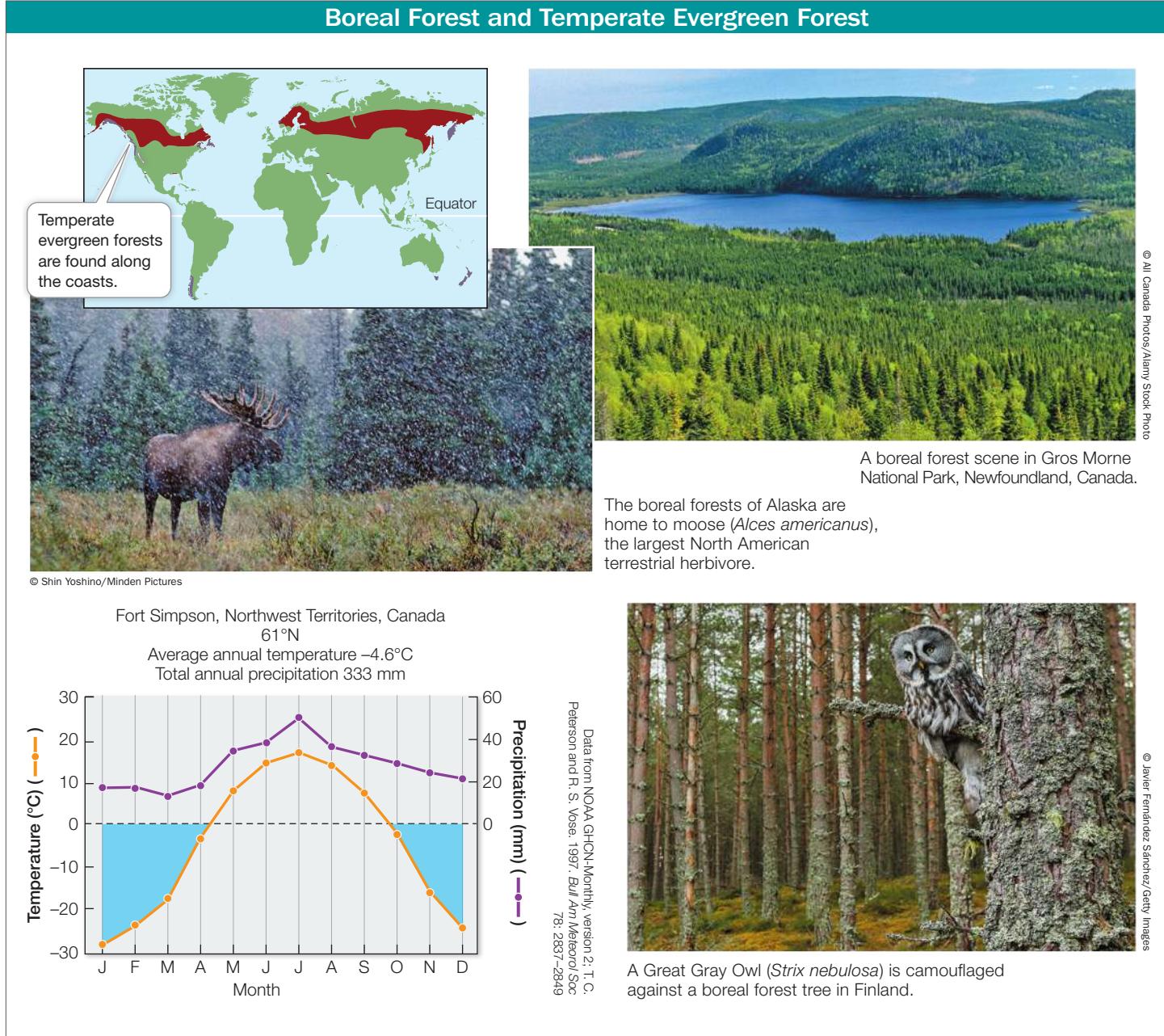
BOREAL FOREST AND TEMPERATE EVERGREEN FOREST The boreal forest biome (also known as taiga) occurs just above 50°N but below Arctic tundra, and at elevations below alpine tundra on temperate-zone mountains. Winters in the boreal forest are long and very cold; summers are short, although often relatively warm. The boreal forests of the Northern Hemisphere are dominated by coniferous trees such as spruces and firs. The short summers favor evergreen leaves, which are ready to photosynthesize as soon as temperatures warm. In winter, downward-drooping limbs allow the trees to shed snow easily.
The dominant mammals of the boreal forest, such as moose and hares, eat leaves, whereas the seeds in conifer cones support a variety of rodents, birds, and insects. Many small mammals hibernate in winter, but voles, lemmings, and mice remain active under the snowpack, serving as food for predators such as foxes and owls.
The temperate evergreen forest biome occurs along the coasts of continents in both hemispheres at middle to high latitudes, where winters are mild and wet and summers are cool and dry. In the Northern Hemisphere, the dominant trees in temperate evergreen forests are conifers, some of which are the world’s most massive tree species (including the giant sequoia and coast redwood). In the Southern Hemisphere, the dominant trees are southern beeches (Nothofagus), some of which are evergreen.
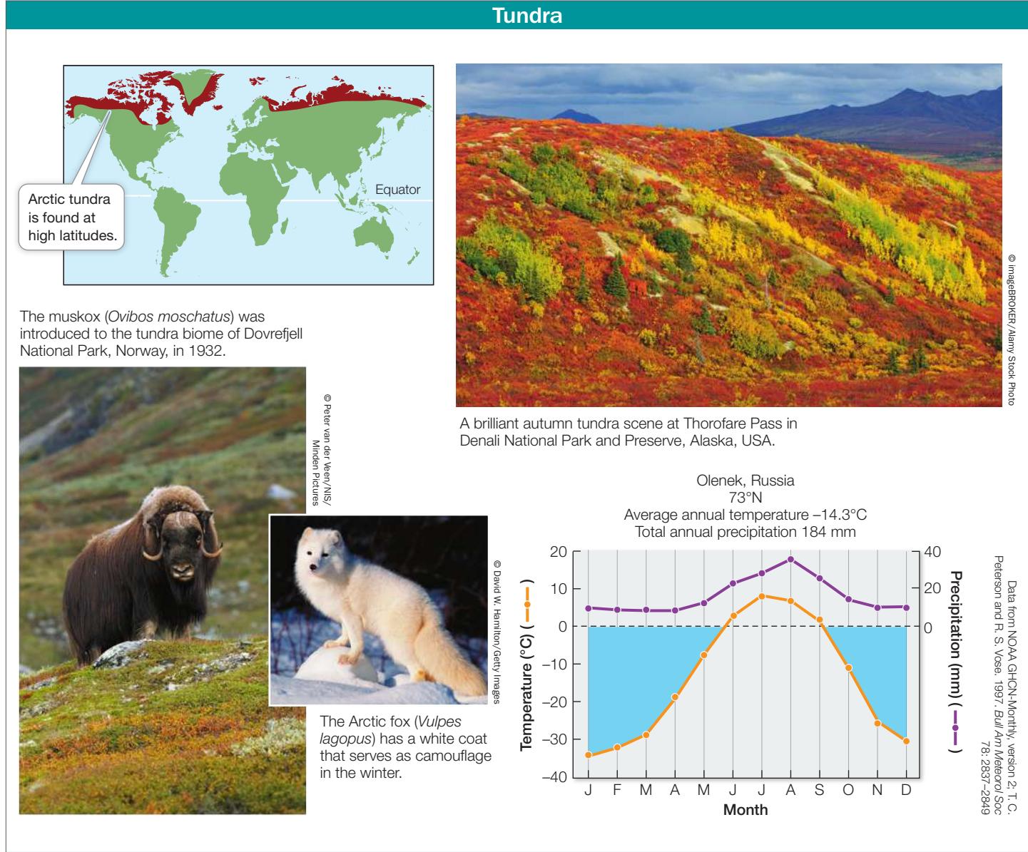
TUNDRA The tundra biome is found at high latitudes (above 65°) characterized by low temperatures and a short growing season. This biome is underlain by permafrost—soil permeated with permanently frozen water. The top few centimeters of the soil thaw during the short summers, when the Sun may be above the horizon 24 hours a day. Thus even though there is little precipitation near the poles, the soil in lowland Arctic tundra is wet because water cannot drain through the permafrost. As a result, trees cannot grow in the tundra biome because their roots cannot penetrate the permafrost. Instead, the tundra biome is characterized by sedges, forbs, grasses, and low-growing shrubs such as heaths, willows, and birches. Lichens and mosses are also important vegetation.
Tundra plants have several structural and physiological adaptations that help them conserve heat, as described in Key Concept 37.1. Most animals are either summer migrants or are dormant for much of the year. Resident birds and mammals, such as the Willow Ptarmigan (Lagopus lagopus) and Arctic fox (Vulpes lagopus), have thick feathers or fur that may change color with the seasons, from brown in summer to white in winter.
Biogeographic regions reflect evolutionary isolation
Climate interacts with local abiotic features to influence where and how organisms live, but these are not the only factors determining where organisms are found. Evolutionary history—where and when species originated and diverged—is key to determining their biogeography.
Until European naturalists traveled the globe in the nineteenth century, they had no way of knowing how organisms were distributed in other parts of the world. Alfred Russel Wallace, who along with Charles Darwin advanced the idea that natural selection could account for the evolution of life on Earth (see Key Concept
19.1), was one of those global travelers. Wallace spent seven years in the Malay Archipelago, where he noticed some remarkable patterns in the distributions of species. For example, he described the dramatically different species that inhabited the adjacent islands of Bali and Lombok. He pointed out that the differences could not be explained by the physical environment, because Bali and Lombok are only 24 kilometers apart.
Wallace saw that, based on the distributions of plant and animal species, he could draw a line that divided the Malay Archipelago into two distinct halves. He correctly deduced that the dramatic differences in flora and fauna were related to the depth of the channel separating Bali and Lombok. This channel is so deep that it would have remained full of water, and thus would have been a barrier to the movement of terrestrial animals, even during the glaciations of the Pleistocene, when sea level dropped more than 100 meters and Bali and the islands to the west were connected to the Asian mainland.
With these insights, Wallace established the conceptual foundations of biogeography. In The Geographical Distribution of Animals, published in 1876, he detailed the factors known at the time that influence the distributions of animals, including past glaciation, land bridges, deep ocean channels, and mountain ranges. He earned some measure of scientific immortality in that the Malay discontinuity that first piqued his curiosity is known to this day as Wallace’s Line (see Figure 52.14).
The biotas of different parts of the world differ enough to allow us to divide Earth into many continental-scale areas called biogeographic regions (Figure 52.14), each containing characteristic assemblages of species. The boundaries of the biogeographic regions in Figure 52.14 were originally proposed by Wallace, and represent assemblages of species that change dramatically, often over short distances. A major process controlling the formation of these biogeographic regions is continental drift. For example, we now know that over the course of the Triassic and Jurassic, the supercontinent Pangaea separated into two great land masses, Laurasia and Gondwana (see Figure 23.14), which subsequently separated into the continents we know today. After the land masses broke up, the descendants of the organisms widely disturbed across Pangaea evolved independently, forming new species and new species assemblages. The legacy of these continental movements can be found in several existing taxonomic groups and in the fossil record. For example, the modern southern beeches—trees of the genus Nothofagus—are found in both the Neotropical and the Australasian biogeographic regions. Evidence of fossilized Nothofagus pollen from 55 to 34 million years ago has also been found in Australia, New Zealand, western Antarctica, and South
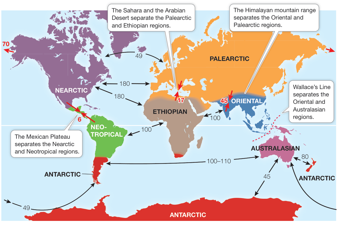
Figure 52.14 Earth’s Biogeographic Regions Wallace identified six major biogeographic regions that are separated by climatic, topographic, or aquatic barriers to dispersal that cause their biotas to differ strikingly from one another. The red arrows on the map show the time (in millions of years) since land masses came together. Black arrows show the time since land masses separated. These areas roughly correspond to Earth’s major tectonic plates. (After H. Kreft and W. Jetz. 2010. J Biogeogr 37: 2029–2053.) Q: As land masses separated, would you expect speciation to increase? Explain.
America, suggesting that beeches originated in Gondwana during the Cretaceous and were geographically separated by the breakup of that land mass 100 million years ago (see Figure 52.14).
Connect the Concepts Key Concepts 23.2 and 23.3 describe how Earth’s land masses have undergone continental drift over the millennia as a result of plate tectonics, shaping major patterns of biogeography.
The evolutionary separation of species can be attributed to two basic processes, vicariance and dispersal. Vicariance occurs when a physical barrier prevents dispersal and divides a species into two or more discontinuous populations. Dispersal occurs when the members of a species cross an existing barrier and establish a new population elsewhere.
Given that the processes of vicariance and dispersal both influence distribution patterns, how can biogeographers determine the role of each process when reconstructing the evolutionary history of a particular species? As you saw in Chapter 20, taxonomists have developed powerful molecular methods of reconstructing the phylogenetic relationships among organisms that can be used to understand how organisms came to occupy their present-day distributions. Phylogenetic trees can be used to discover whether the distribution of an ancestral species was influenced by a vicariant event, such as continental drift or a change in sea level, or was simply the result of a dispersal event.
Diversity varies with latitude and longitude
About 200 years ago, the German explorer and naturalist Alexander von Humboldt spent 5 years traveling around Latin America. He remarked in the account of his voyages that “the nearer we approach the tropics, the greater the increase in the variety of structure, grace of form, and mixture of colors, as also in perpetual youth and vigour of organic life.” Humboldt and other nineteenth-century scientific explorers such as Wallace and Darwin became keenly aware of this pattern as they collected thousands of species in the tropics and compared them with their more meager collections from Europe. As more observations and collections have been made over the last 200 years, the latitudinal gradient in species diversity has been established for a wide variety of taxa, including some groups of birds, mammals, flowering plants, and insects such as swallowtail butterflies (Figure 52.15A). Significant variation in species diversity is also seen with longitude, but the number of species depends largely on the longitudes chosen.
There are intriguing exceptions to the classic latitudinal patterns of species diversity just described. Some taxa show a positive relationship between species number and latitude (Figure 52.15B). That is, among some taxa—for example, seabirds—species number increases at higher latitudes. This pattern of seabird diversity correlates with marine net primary productivity, which is substantially higher in temperate and polar oceans than in the tropics.
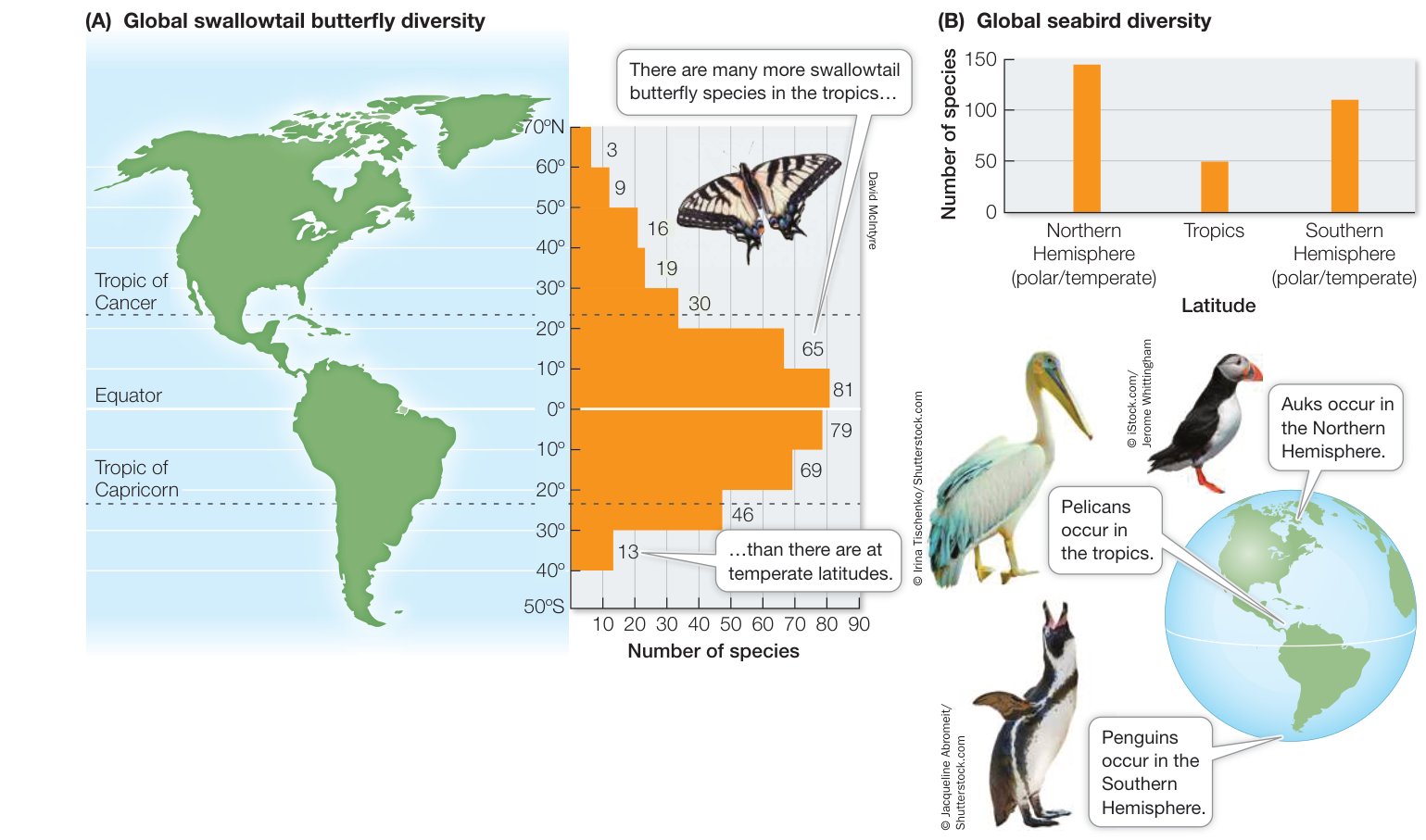
Figure 52.15 Latitudinal Gradients in Diversity (A) Among swallowtail butterflies (Papilionidae), species richness decreases with latitude both north and south of the equator. (B) Seabirds, by contrast, show a positive relationship between species diversity and latitude: the number of seabird species increases at higher latitudes. (A after J. M. Scriber. 1973. Psyche 80: 355–373; B graph data from P. Harrison 1987. A Field Guide to Seabirds of the World. Penguin Random House: London.)
Connect the Concepts Key Concept 56.2 describes net primary production (NPP) as the amount of biomass incorporated into the tissues of primary producers and as the base of all food chains.
We consider productivity differences along with other explanations of latitudinal gradients in diversity in the next section.
Geographic variation in diversity is explained by multiple factors
Although most ecologists agree that latitudinal gradients in diversity exist, there is much less consensus as to why they exist. Dozens of hypotheses have been proposed to explain these patterns, but they are hard to evaluate—in part because there are multiple and confounding differences in such factors as geographic area, climate, and productivity with latitude. More important, because these factors operate at large spatial scales and over evolutionary time, it is impossible to conduct experiments to isolate the factors and separate correlation from causation.
Here we present three well-known hypotheses that have been advanced to account for latitudinal gradients in diversity. Corroborative evidence can be found for each of these hypotheses, varying with taxon, locality, and scale, which suggests that none of these hypotheses is mutually exclusive. Multiple factors, working at multiple spatial scales, are likely responsible for common biogeographic patterns.
SPECIES DIVERSIFICATION RATE This hypothesis proposes that in the tropics the rate of speciation is higher and the rate of extinctions is lower, resulting in overall higher species diversity than in temperate or polar regions. Two factors could account for a higher speciation rate in the tropics: a larger geographic area (this is the widest part of the planet, so it encompasses the greatest amount of area) and a warm and stable climate. The rationale is that a larger geographic area with a consistent climate should promote speciation because species will have larger geographic ranges, giving them a greater chance of reproductive isolation (see Key Concept 22.2). In addition, these large and stable areas should reduce extinctions. The net result should be an increase in the number of species in the tropics.
SPECIES DIVERSIFICATION TIME This hypothesis proposes that the amount of time over which speciation has taken place is greatest in the tropics—in other words, that the tropics have a longer evolutionary history than temperate or polar regions. First championed by Wallace in 1878, this hypothesis proposes that tropical regions, because they are more climatically stable over time, have more time to diversify than temperate or polar regions, where severe climate conditions (such as ice ages) could have decreased speciation and increased extinction. Thus even if the rates of speciation and extinction are the same worldwide, the tropics should have accumulated more species over time simply because of the lack of dramatic changes in climate.
PRODUCTIVITY This hypothesis proposes that species diversification is promoted by higher productivity, which allows species more resources and thus decreased risk of species extinction due to competition. The productivity hypothesis might explain the positive relationship between seabird diversity and increasing latitude, given that ocean productivity is generally higher at temperate and polar latitudes. As you will see in Chapter 55, the role of productivity can more easily be explored at smaller spatial scales, where experiments can give us a better idea of its role in determining species diversity.
Recap and Assess
Biogeographic patterns are interconnected across a hierarchy of scales ranging from global to local. Three strong biogeographic patterns can be seen: (1) biomes, or groupings of ecologically similar organisms, are shaped by the environment, (2) diversity varies from continent to continent, forming biogeographic regions, and (3) diversity varies with latitude.
- What are the differences and similarities between the tropical rainforest biome and the temperate evergreen forest biome?
- Refer to Figure 52.14. Why did Wallace’s Line help explain what controls the formation of biogeographic regions?
- Over Earth’s history, ice sheets extended into temperate latitudes. Does this fact better support the species diversification rate or the species diversification time hypothesis proposed to explain latitudinal variation in diversity? Explain.
As you have seen, an important aspect of biogeography is the relationship between diversity and geographic area. We have considered this relationship at global scales. We turn now to smaller regional scales, to understand in more detail the importance of geographic area to patterns of biogeography.
Geographic Area and Humans Affect Regional Species Diversity
Learning Objectives
- 52.5.1 Discuss the species–area relationship and use the theory of island biogeography to explain the pattern.
- 52.5.2 Describe how humans have affected biogeographic patterns.
- 52.5.3 Describe specific ways in which habitat fragmentation negatively affects species diversity.
Biogeographers have repeatedly documented what is termed the species–area relationship, in which species diversity increases with increasing area. The relationship has most often been measured for islands or islandlike habitats—any isolated area surrounded by a “sea” of dissimilar habitat. In addition to showing a pattern of increasing species diversity with increasing area, islands also show a pattern of decreasing species number with distance from the source of those species, or the species pool (Figure 52.16). How do island area and distance act together to produce species–area relationships?
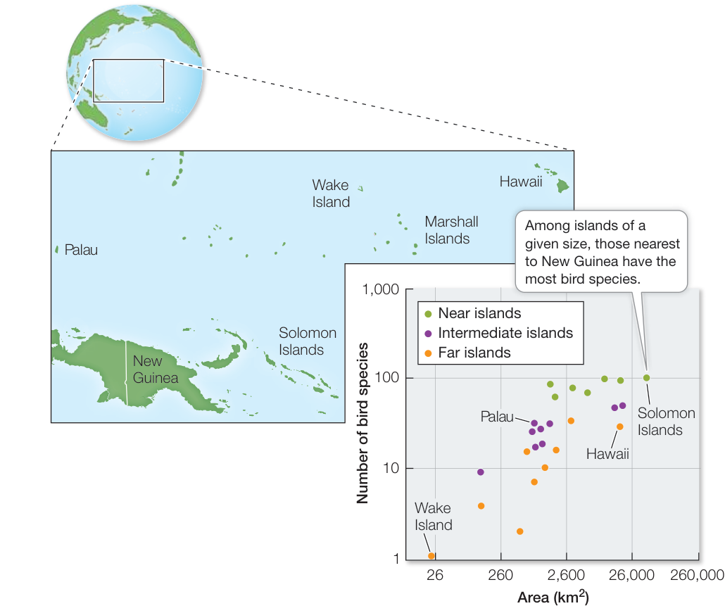
Figure 52.16 The Species–Area Relationship E. O. Wilson and Robert MacArthur plotted the number of species of birds against the size and distance of islands from New Guinea. Larger and closer islands consistently contained more species, a fact that these scientists incorporated in their theory of island biogeography. (After R. H. MacArthur and E. O. Wilson. 1963. Evolution 17: 373–387.)
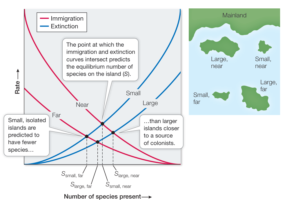
Figure 52.17 The Equilibrium Theory of Island Biogeography MacArthur and Wilson’s theory emphasized the balance between species immigration rates and species extinction rates for islands of different sizes and at different distances from a source of colonizing species. (After R. H. MacArthur and E. O. Wilson. 1963. Evolution 17: 373–387.)
The biologist Edward O. Wilson was struck by the species–area relationship from his research on ant biogeography and was looking for explanations. He teamed up with Robert MacArthur, a gifted mathematical ecologist, to develop the theory of island biogeography to explain this pattern. They based their theory on just two processes: the immigration of new species to an island and the extinction of species already present on that island (Figure 52.17). The premise of island biogeography is that the number of species on an island represents a balance between the rate at which species immigrate to and colonize the island and the rate at which resident species become locally extinct.
The rate of immigration is determined in part by the number of species in the regional species pool. In the case of oceanic islands, the species pool comprises all the species on the nearest mainland location. Not all species that reach the island will persist there, however. The more species there are on an island, the greater the likelihood that some will go extinct, either due to chance or the inability to coexist with other species on the island. The number of species that will be sustained on any particular island is determined by the balance of the immigration rate and the extinction rate for that island. Even though species will come and go over time (i.e., immigrate and become extinct), that turnover will always result in some equilibrium number of species, assuming a constant species pool and natural extinction events.
The actual number of species on an island will ultimately depend on two factors:
- The size (area) of the island. The smaller the island, the fewer resources it provides, the greater the potential for competition, and the higher the extinction rate will be (see Figure 52.17). Larger islands provide more resources and can sustain larger populations (which tend to have lower extinction rates than small populations).
- Distance of the island from the species pool. The farther the island is from the source of immigrants, the lower the immigration rate—the rate at which new species arrive—will be (see Figure 52.17).
Between 1966 and 1969, Wilson and his student Daniel Simberloff conducted an experiment to test the theory of island biogeography, using arthropods living on mangrove islands in the Florida Keys. You can view this experiment and the results online.

Animation 52.3 Island Biogeography in the Florida Keys
Humans exert a powerful influence on biogeographic patterns
The theory of island biogeography has provided surprising insight into the role human’s play in regional biogeographic patterns. As you saw in Key Concepts 52.3 and 52.4, Earth’s biomes are becoming smaller and more fragmented by local-and regional-scale forces such as agriculture, deforestation, and urbanization. They are being transformed into islandlike habitats—isolated patches of suitable habitat such as parks or forest fragments, surrounded by extensive areas of unsuitable habitat similar to the cattle pastures of Amazonia described at the opening of this chapter.
The fragmentation of the Amazon rainforest led Thomas Lovejoy and his colleagues to initiate, in 1979, one of the largest and longest-running ecological experiments ever conducted to investigate the effects of tropical forest fragmentation on species diversity (Investigating Life: The Largest Experiment on Earth). The Biological Dynamics of Forest Fragments Project (BDFFP) took
Investigating Life: The Largest Experiment on Earth
Experiment
Original Paper: G. Ferraz et al. 2003. Rates of species loss from Amazonian forest fragments. Proc Natl Acad Sci USA 100: 14069–14073. © 2003 National Academy of Sciences U.S.A.
Thomas Lovejoy and his colleagues asked what was the minimum area needed to maintain species diversity in the rainforest fragments created by logging near Manaus, Brazil. They conducted an experiment, starting in 1979, that took advantage of an existing Brazilian law that required landowners who cut rainforest to leave half of it untouched. In 2003, Ferraz and colleagues reported on one particular aspect of the experiment: the number of forest understory birds living in different-sized forest fragments surrounded by deforested land.
HYPOTHESIS The number of understory bird species will decline faster after the isolation of the fragment, and in smaller rainforest fragments compared with larger rainforest fragments.
METHOD
- Starting in 1979, fragments of three sizes (1, 10, and 100 ha) were established 80 km north of Manaus. The fragments were separated from continuous forest by at least 100 meters of cleared land.
- Birds were captured in mist nests placed in the fragments prior to deforestation and then for 12 years after fragment establishment. The mist nets were placed in roughly the same locations throughout the study.
- Each newly captured bird was recorded for species, given an individually numbered band, and released back into the rainforest from which it was caught.
- The data gathered were used in species-loss curves for each fragment, and a scaling factor (i.e., a number that scales, or multiplies, by some quantity) was estimated to determine the time it takes to lose half of the bird species () in fragments of different sizes.
Animation 52.4 Edge Effects
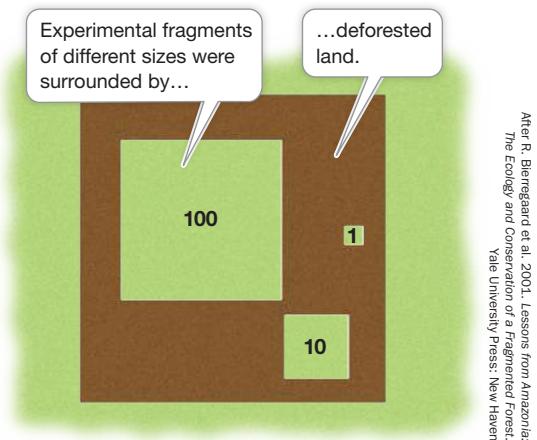
After R. Bierngaard et al. 2001. Lessons from Amazonia: The Ecology and Conservation of a Fragmented Forest. Yale University Press: New Haven
RESULTS The average initial number of species was 83 for the 1-ha fragment, 92 for the 10-ha fragment, and 113 for the 100-ha fragment. Despite finding a total of 164 understory bird species in the fragments over the course of 13 years, there was a significant drop in the number of species over time. The was shortest in the 1-ha fragments and longest in the 100-ha fragments. Fragments of 100 ha were predicted to lose half of their species in 12 years.
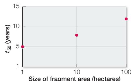
CONCLUSION The number of understory bird species declined after the fragmentation of tropical rainforest habitat by deforestation. Smaller rainforest fragments lost species faster than larger forest fragments. Even the largest fragments were predicted to lose half of their bird species.
Investigating LIFE Work with the Data follows on the next page.
Work with the Data
The data in the graph shown in the experiment can be used to calculate a scaling factor for the time it takes to lose half of the bird species within a fragment. The scaling factor shows that to increase the (i.e., the time it takes fragments to lose half their species) by 10-fold, fragment area would need to increase 1,000-fold. Here you will use this scaling factor and other data provided in the graph to determine the area needed for the conservation of understory birds in the Amazon forests outside Manaus, Brazil.
QUESTIONS►
Graph the initial numbers of bird species by the size of the fragment area. Do these fragments follow the species-area relationship?
- Suppose you are consulting for the Brazilian government on the conservation of rainforests near Manaus. Assuming that the for 1 ha is 5 years, what is the minimum size that a rainforest fragment in the Manaus area needs to be to ensure that half of the bird species remain 50 years after the deforestation event that isolated them? How about a century after deforestation?
- Suppose it takes 100 years for rainforests to fully recover after a deforestation event in the Manaus region. Given that the average size of a rainforest fragment in this area is no bigger than 1,000 ha, will the number of species decline by half before the recovery of rainforest occurs around the largest fragments?
advantage of an existing Brazilian law that required landowners who cut rainforest to leave half of it untouched. Lovejoy was able to survey the species diversity in different-sized fragments (either 1, 10, or 100 hectares [ha] in size surrounded by deforested land). Among several results, his group found that, after more than 30 years of isolation, even the largest deforested fragments surveyed (100 ha) had lost half of their bird species diversity. The researchers were also surprised by two additional findings. First, even minimal distances of 80 meters between fragments resulted in strong avoidance of the clearings, and thus isolation, by birds, insects, and tree-dwelling mammals that lived in the fragments. Second, the fragmentation exposed species within a fragment to a variety of potential hazards, including extreme heat, fires, hunting, predators, diseases, and invasive species. These so-called edge effects not only reduce the immigration rate from one fragment to another, thus contributing to a smaller species pool, but they effectively reduce the size of the fragment, thus increasing the extinction rate, by making the edge of the fragment much less hospitable habitat.
Recap and Assess
Species-area relationships, in which species diversity increases with increasing area, have been shown for islands and islandlike habitats. Smaller islands have higher extinction rates and lower immigration rates compared with larger islands. Earth’s biomes are becoming smaller and more fragmented by human activities, leading to lower diversity in the remaining habitats.
- Why do island size and distance from a species pool affect island biogeography?
- Why is habitat fragmentation by human activities threatening species diversity? Besides ceasing the activity altogether, what can be done to reduce this threat?
Investigating Life: QA How do geographic area and isolation affect the biogeography of life on Earth?
At the opening of the chapter, we asked how geographic area and isolation might affect the biogeography of life on Earth. You have seen that this question is highly relevant at different spatial scales—from whole continents to small islands—and also over different time scales—from millions of years to months. Because the spatial and temporal scales at which biogeographic patterns manifest themselves are so wide and interconnected, it can be hard to test theories of biogeography with experiments that are large and long enough to be meaningful. The Biological Dynamics of Forest Fragments Project (BDFFP), an experiment conducted in the most species-rich region of the world, and at arguably the largest scale ever attempted, offers support for theories proposed nearly 200 years ago by explorers such as Humboldt, Wallace, and Darwin, who hypothesized that the distribution of species on Earth is highly influenced by the geographic area and isolation those species have experienced. The question remains, in the case of the Amazon Basin, whether species will ultimately adapt to the changing biogeographic landscape or become a casualty of an extinction event that would be unrivaled in human history.
Future directions
One of the major findings of the BDFFP is the importance of connectivity in maintaining species diversity. Management and permitting of forest clearing are focusing on creative ways to connect forest fragments by taking advantage of existing landscape features to increase connectivity of disturbed habitat. For example, in Amazonia strong laws exist to prohibit clearing forest along rivers and steep slopes, providing strips of land that can serve to connect fragments around newly cleared land.
© Morley Read/Alamy Stock Photo
You should be able to relate each summary to the adjacent figures. If you go to this visual summary in Achieve, you can follow links to figures, animations, activities, and simulations that will help you consolidate the material.
Visual Summary
Ecology Is the Study of the Interrelationships among Organisms and the Environment
- ■ Ecology differs from environmentalism, which involves the use of ecological knowledge to inform our stewardship of natural resources.
- ■ Ecologists have a use-inspired focus to their research, motivated by a desire to address Earth’s ecological problems.
- ■ Ecology is studied at multiple levels of organization, ranging from individuals to the biosphere.
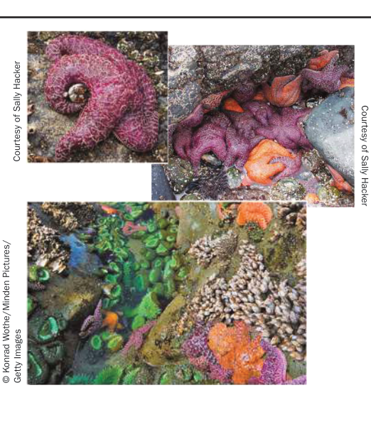
Figure 52.1
Questions
- Define the difference between ecology and environmentalism.
- What is meant by “use-inspired” ecological research?
- How are individuals connected to communities?
Global Climate Is a Fundamental Component of the Physical Environment
- ■ Climate and weather both refer to atmospheric conditions, but climate represents conditions over years to millennia whereas weather represents conditions over days to weeks.
- ■ Solar radiation drives global climate. Of the solar radiation that hits Earth, some is reflected back to space (30%) and the rest is absorbed by the atmosphere (20%) or by Earth’s surface (50%). Greenhouse gases trap heat radiating back out toward space.
- ■ Latitudinal differences in solar energy input drive patterns of atmospheric circulation.
- ■ The interaction of Earth’s rotation and north-south air mass movements generate prevailing winds, which in turn drive ocean currents.
- ■ The seasons are a consequence of Earth’s tilt and orbit around the Sun.
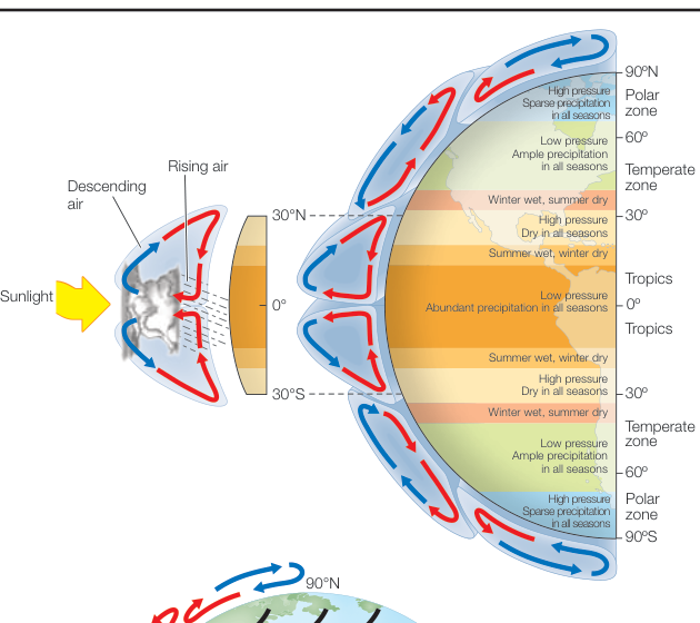
Figure 52.5 1. 1. Does a week of extreme cold weather tell us that Earth’s climate is not warming? 2. 2. Why are the tropics warm and wet and the poles cold and dry? 3. 3. What direction do ocean currents flow as a result of trade winds?
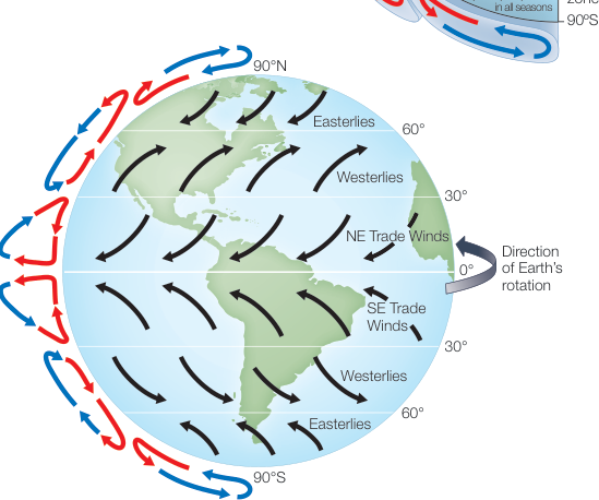
Figure 52.6
- ■ Earth’s land topography creates rain shadows and temperature inversions, producing variation in temperature and precipitation.
- ■ Ocean-floor topography affects water depth, which affects light penetration and water temperature, pressure, and movement, creating aquatic zones and ocean upwelling.
- ■ Vegetation, especially forests, affects climate through the process of evapotranspiration.
- ■ Humans have transformed their environment, including urban climate.
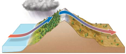
Figure 52.9
Questions
- How does a rain shadow affect climate on either side of a mountain range?
- How do winds and ocean-floor topography create ocean upwelling?
- Why would planting more trees in an urban area help with urban climate warming?
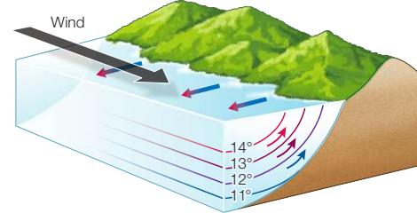
Biogeography Is the Study of How Organisms Are Distributed on Earth
- ■ Patterns of biogeography are interconnected across a hierarchy of scales, ranging from global to regional to landscape to local.
- ■ Terrestrial biomes are groupings of ecologically similar dominant plants shaped by patterns of temperature and precipitation.
- ■ Earth’s diversity varies from continent to continent, forming biogeographic regions and reflecting evolutionary isolation as a consequence of Earth’s geological history.
- ■ Earth’s diversity varies with latitude. Hypotheses explaining this variation rely on multiple factors, including geographic area, time, climate, and productivity.
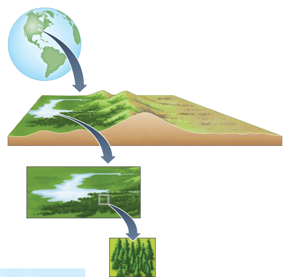
Figure 52.12
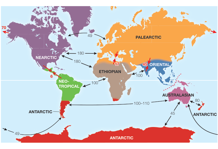
Figure 52.14
Geographic Area and Humans Affect Regional Species Diversity
and Simulation 52.1
- ■ Species-area relationships, in which species diversity increases with area, have been shown for islands and area fragments.
- ■ The theory of island biogeography states that the number of species on an island is a balance between immigration and extinction rates, which vary by island size and distance from the species pool.
- ■ As humans fragment Earth’s biomes through agriculture, deforestation, and urbanization, remaining habitats become more isolated, or islandlike.
Questions
- Describe why species diversity increases with increasing island or fragment area.
- Using Figure 52.17, explain why the small and far islands have lower species numbers than the large and near islands.
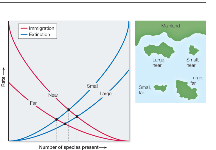
Figure 52.17