Chapter 53Populations
Key Concepts
- 53.1 Populations Show Dynamic Variation in Size over Space and Time
- 53.2 Population Growth Describes the Change in Population Size over Time
- 53.3 Life History Is the Lifetime Pattern of Growth, Reproduction, and Survival
- 53.4 Population Biology Can Be Used in Managing and Conserving Populations
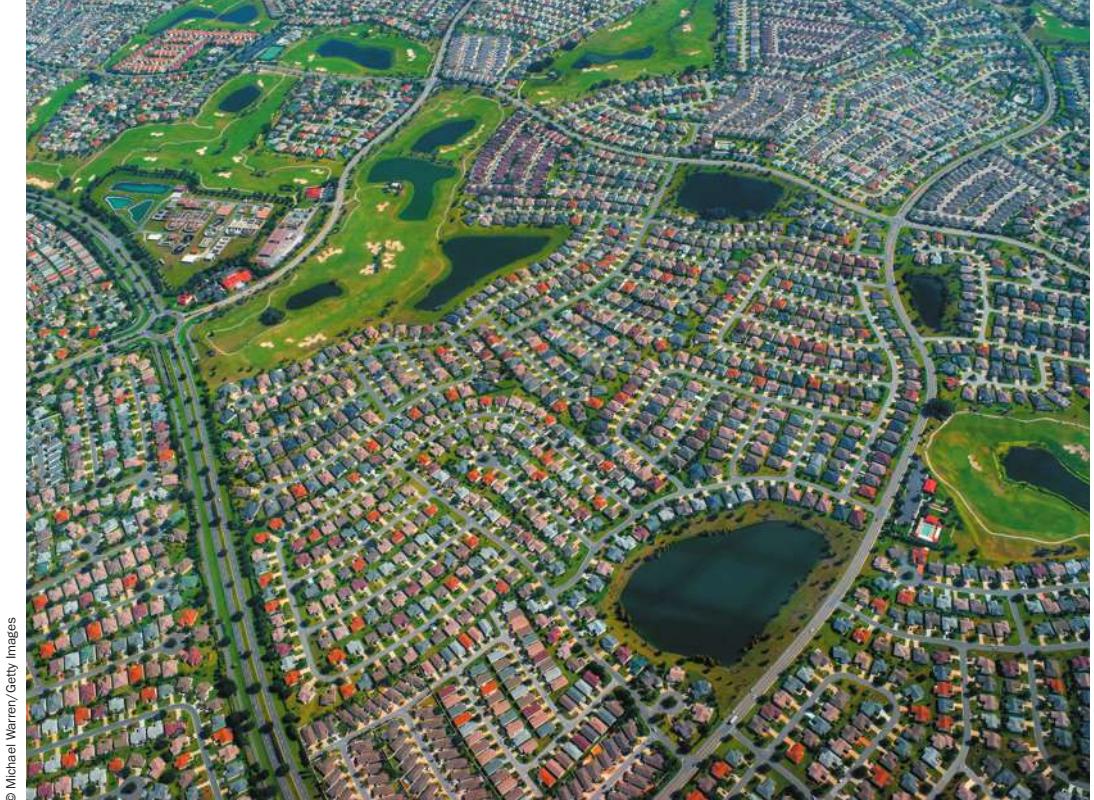
The human population crossed the 7.7 billion mark in 2019.
© Michael Warren/Getty Images
Investigating Life: Earth’s Human Carrying Capacity
In 1798 Thomas Robert Malthus, in his Essay on the Principle of Population, pointed out that the human population was growing exponentially but its food supply was not, and argued that at some point, famine and death would be the ultimate fate of the human race. Malthus could not have anticipated the technological innovations over the next 200 years that would greatly enhance our food production and health care. Today, however, the size of the human population is once again a serious concern as we confront the effects of our contributions to climate change, pollution, habitat destruction, and species extinctions.
For thousands of years, Earth’s capacity to support human populations was low because of the relative inefficiency with which we could obtain food and water. The development of social systems and communication, the domestication of plants and animals, ever-increasing crop and livestock yields due to ongoing technological advances, and our increasing proficiency at managing diseases all contributed to unprecedented growth of the human population. It took more than 200,000 years for the human population to reach 1 billion people, which happened in the early nineteenth century. Today, a mere 200 years later, the planet is home to roughly 7.7 billion human beings.
Many believe that human populations will (if they have not already) reach some maximum size (known as the population’s carrying capacity) above which continued population growth is unsustainable. Food production is critical to human population growth and currently uses large amounts of land, water, fertilizers, and energy. Housing and quality health care require advances in infrastructure and drug production, and these too are highly energy-intensive. In addition, if Earth’s ecosystems continue to be degraded by climate change, human populations may experience a general breakdown of Earth’s life support systems.
Luckily, population growth rate has slowed from its high after World War II, but with a base of 7.7 billion, even minimal population growth rate means millions more individuals each year. As you will see later in the chapter, population biologists have used census data and standard population growth models to predict human population sizes into the future.
QA What is the human population growth projected to be in the next century, and how will that affect population size? (Find the answer on page 1214.)
Populations Show Dynamic Variation in Size over Space and Time
Populations Show Dynamic Variation in Size over Space and Time
Learning Objectives
- 53.1.1 Describe how species are divided into populations, metapopulations, and geographic ranges.
- 53.1.2 Describe how populations vary in space and time and compare the three main factors that control population dynamics.
- 53.1.3 List and describe major approaches that ecologists use to estimate population size and extent.
Species, whether they are humans, yeast, or giant redwood trees, are divided into groups of individuals, or populations. A population is a group of individuals of the same species within a given area that have the potential to interbreed and interact with one another. As you might expect, populations vary in their population size—the numbers of individuals within a population. Well before ecology became a distinct biological discipline, humans were interested in population dynamics, the patterns and processes of population change over space and time. Growing crops, raising livestock, and controlling pests all involve paying attention to population dynamics. To this day, game wardens, park managers, and conservation biologists aim to maintain stable populations of fishes, wildlife, and threatened or endangered species in the face of change. Here we consider population dynamics in more detail.
Part of the dynamism that populations show is a consequence of their distribution across the landscape (Figure 53.1A). For example, distribution maps of the herbaceous perennial Clematis fremontii
show that it is patchily distributed across Missouri, Kansas, and Nebraska. Here populations are restricted to dry, rocky meadows formed on particular limestone outcrops within the region. Populations, such as those of Clematis, rarely occur in isolation from one another and are usually connected through dispersal. Dispersal is simply the movement of individuals into (immigration) or out of (emigration) an existing population. A group of geographically isolated populations linked together by dispersal is known as a metapopulation. For example, a cluster of meadows might be considered a metapopulation if Clematis seeds from one meadow had the potential to disperse to another meadow. At larger spatial scales, the entire geographic range, or distribution, of a species might consist of one or multiple metapopulations, depending on the extent of the area occupied by a species.
Species differ greatly in their geographic ranges—they can be as wide-ranging as the acorn barnacle Semibalanus balanoides, which extends along both North American coasts and the European Atlantic coast. However, even though dispersal links populations, most species have fairly restrictive geographic ranges, such as we see for Clematis. We call such species endemic because they occur in one particular location and nowhere else on Earth. Thus Clematis can be said to be endemic to the central United States because its geographic range is restricted to that region.
Within a population, the spatial arrangement of individuals may vary in what are known as dispersion patterns. Ecologists recognize three basic dispersion patterns: (1) regular (or uniform) dispersion, characterized by evenly spaced individuals, (2) random dispersion, in which individuals are randomly spaced, and (3) clumped dispersion, in which individuals tend to be clustered in groups (Figure 53.1B). As we will consider later in this key concept, multiple processes such as resource availability, species interactions, and dispersal can shape the dispersion patterns we see in nature.
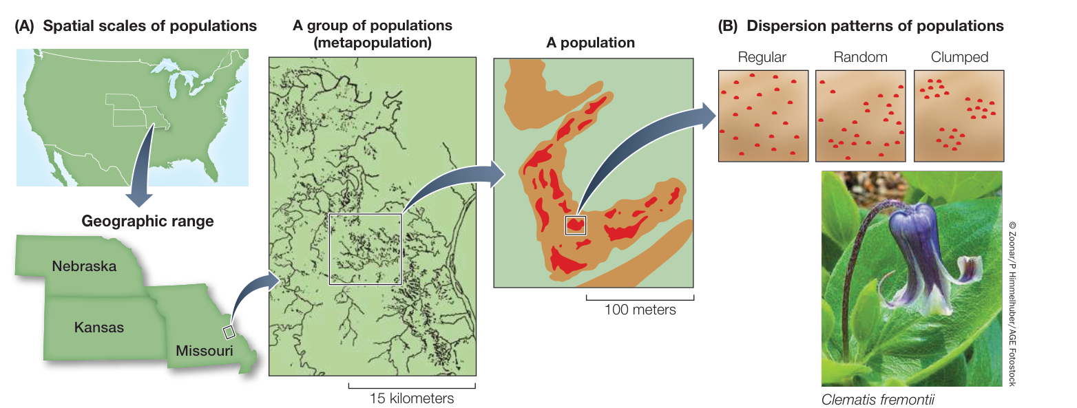
Figure 53.1 Many Populations Have Patchy Distributions The abundance of the herbaceous perennial Clematis fremontii is patchy over different spatial scales. (A) Populations occur within limestone meadows. A group of populations makes up a metapopulation, and multiple metapopulations make up the geographic range (in this case, Missouri, Kansas, and Nebraska). (B) Individuals within a population show one of three different dispersion patterns. (A after R. Erickson 1945. Ann MO Bot Gard 32: 413–460.)
Populations can vary over time as well. For example, some populations may show “boom and bust” cycles, such as we see for bacteria, yeast, and phytoplankton, in which the population size can vary over just a few minutes to days. Species that show wide fluctuations in population size tend to have reproductive strategies that allow them to respond rapidly to changing resources. They may also have predators that are able to take advantage of these outbursts in growth. For example, aphids engage in parthenogenetic reproduction—a type of asexual reproduction resulting in genetically identical individuals—which allows them to become very abundant very quickly. If overcrowding occurs and food resources become limiting, populations can crash, leaving behind a few individuals that may ultimately serve to increase the population size through rapid clonal reproduction (Figure 53.2). Predatory insects such as the insidious flower bug can dampen these large swings in aphid population size, resulting in decreased resource limitation. Thus extrinsic factors such as predation can provide checks on populations, thereby limiting outbreaks.
Population dynamics are controlled by the physical environment, biological interactions, and dispersal
Even though we know that populations fluctuate in space and time, determining the factors responsible for this variation can be challenging. Ecologists recognize three main factors that affect population dynamics and that act simultaneously to set limits for populations and species: the physical environment, biological interactions, and dispersal.
As you saw in Chapter 52, the distribution and abundance of species are highly dependent on the physical environment; factors such as climate, topography, and even human infrastructure set physiological limits for species. Thus it makes sense that the physical features of the environment strongly limit a population’s geographic extent and size through time. You saw this for Clematis, whose populations are restricted to dry, rocky limestone soils, resulting in a patchy distribution pattern (see Figure 53.1).
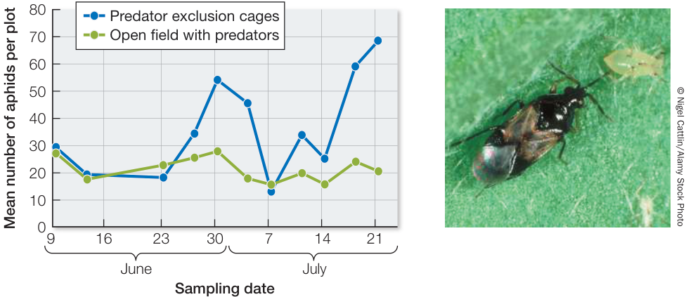
Figure 53.2 Population Fluctuations of Aphids and Their Predators A population of soybean aphids (Aphis glycines) fluctuates more when its insect predator, the insidious flower bug (Orius insidiosus), is excluded than when it is present. Without the predator, soybean aphids cost soybean growers hundreds of millions of dollars in damage per year. (Graph after N. Desneux et al. 2006. Environ Entomol 35: 1342–1349.)
Likewise, many types of biological interactions affect population dynamics. Interbreeding among individuals within populations affects their size and extent—in fact, many populations can be defined by the genetic similarity of the individuals within a given area (see Key Concept 19.4). For example, populations of wild endangered salmon, which look nearly identical to hatchery-raised salmon, can be assessed for population size using genetic techniques that allow differentiation among populations. In addition, because individuals within populations share similar resources, intraspecific competition (competition for shared resources by individuals of the same species) can be critical in controlling population size, as you will see in Key Concept 53.2. Interspecific interactions (interactions among individuals of different species) are another important factor in controlling population dynamics.
Connect the Concepts Chapter 54 describes how interspecific interactions such as competition, predation, and positive interactions (i.e., mutualisms and commensalisms) often set the upper limits on the number of individuals within populations.
Finally, dispersal can be a critical factor controlling population dynamics. Dispersal comes in many forms. It can be active when movement is controlled by the individual, such as you might see with elephants; passive when movement is controlled by the physical environment, as in corals and dandelions; or facilitated by active agents, such as birds or bats dispersing seed-laden fruits (Figure 53.3). Dispersal is a mechanism that can reduce competition for resources, either with a parent or another individual within the population. In addition, dispersal allows individuals to escape a harsh physical environment. Thus dispersal serves as a mechanism to reduce the probability of local extinctions of populations by spreading the risk among multiple populations that are geographically separated (see Key Concept 53.4).
A specific type of dispersal is migration. Migration typically occurs in response to seasonal variation in resources, involves round-trip movement, and includes the whole population. For example, North Pacific populations of the humpback whale migrate more than 4,800 kilometers between their winter breeding grounds in the south (Mexico, Hawaii, and Japan) and their summer feeding grounds in the north (Northeast Pacific coast and Gulf of Alaska) (Figure 53.4). Scientists determine whale migration patterns and population numbers by taking photographs and collecting genetic material to follow and compare individuals in the feeding and breeding grounds. A 2006 survey of North Pacific humpback whales determined that close to 20,000 individuals in five separate populations make the migration every year. Remarkably, there were only 1,400 North Pacific humpback whales in 1966, when commercial whaling of these populations was banned.
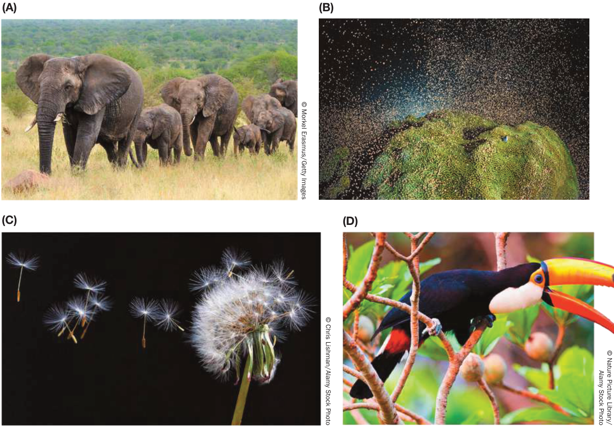
Figure 53.3 Different Dispersal Mechanisms of Organisms (A) Elephants actively disperse, (B, C) corals and dandelions disperse passively, and (D) seeds within fruits are typically dispersed by an active agent, in this case a Toco Toucan (Ramphastos toco).
As you can see, whale biologists use various techniques to estimate the population sizes of humpback whales. Let’s consider in more detail the variety of approaches ecologists use to measure population size.
Ecologists use a variety of approaches to estimate population size and extent
Accurately measuring the size and extent of a population is harder than you might think. One challenge is determining the boundary of the population. If the area is self-contained and small enough, you might be able to simply count all the individuals of a particular species to get the population size. Biologists performed this type of count, called a full census, on the African bush elephant (Loxodonta africana) population of Samburu and Buffalo Springs National Reserves in Kenya. By monitoring the elephants for 21 months, the biologists learned to recognize each of the 760 individuals in the population, primarily by their unique and distinctive ear markings. But populations are often too large and too mobile for a full census; often the extent of the range of a population is not perfectly known. In these cases, ecologists instead determine the population density, or the number of individuals within a given area (or volume, for organisms living in water), and then extrapolate from these samples to estimate the total population size.
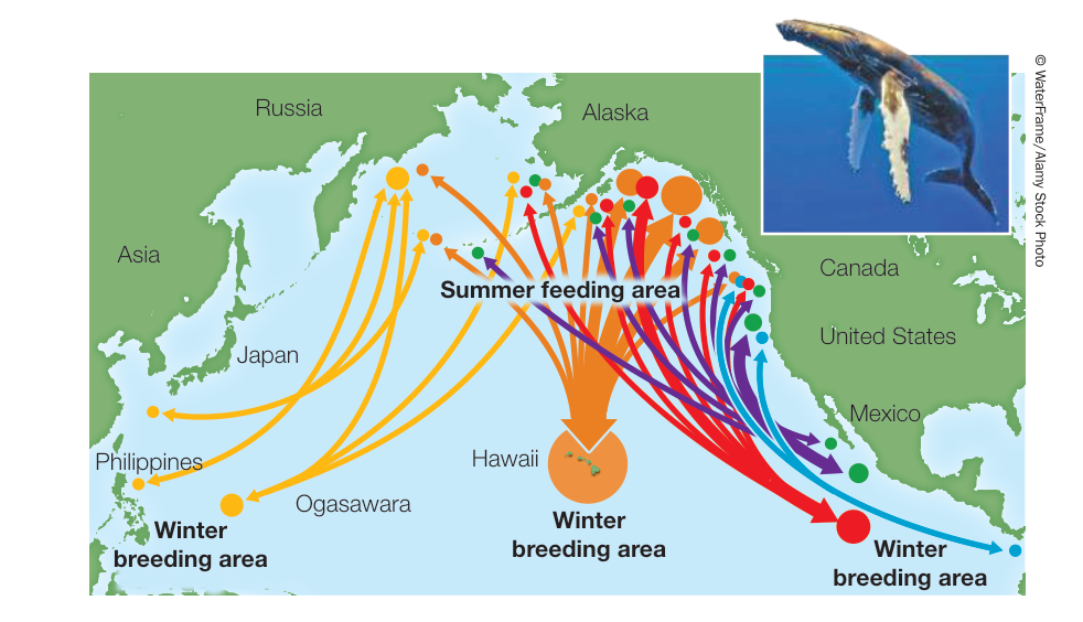
Figure 53.4 Migration of North Pacific Humpback Whales North Pacific populations of the humpback whale (Megaptera novaeangliae) migrate between their winter breeding grounds off Mexico, Hawaii, and Japan and their summer feeding grounds in the Gulf of Alaska and Northeast Pacific coast. A 2006 survey of North Pacific humpback whales determined that close to 20,000 individuals migrate in five separate populations (represented by different colored arrows). (After https://hawaiihumpbackwhale.noaa.gov/explore/humpback\_whale.html. Migration data from SPLASH Research.)
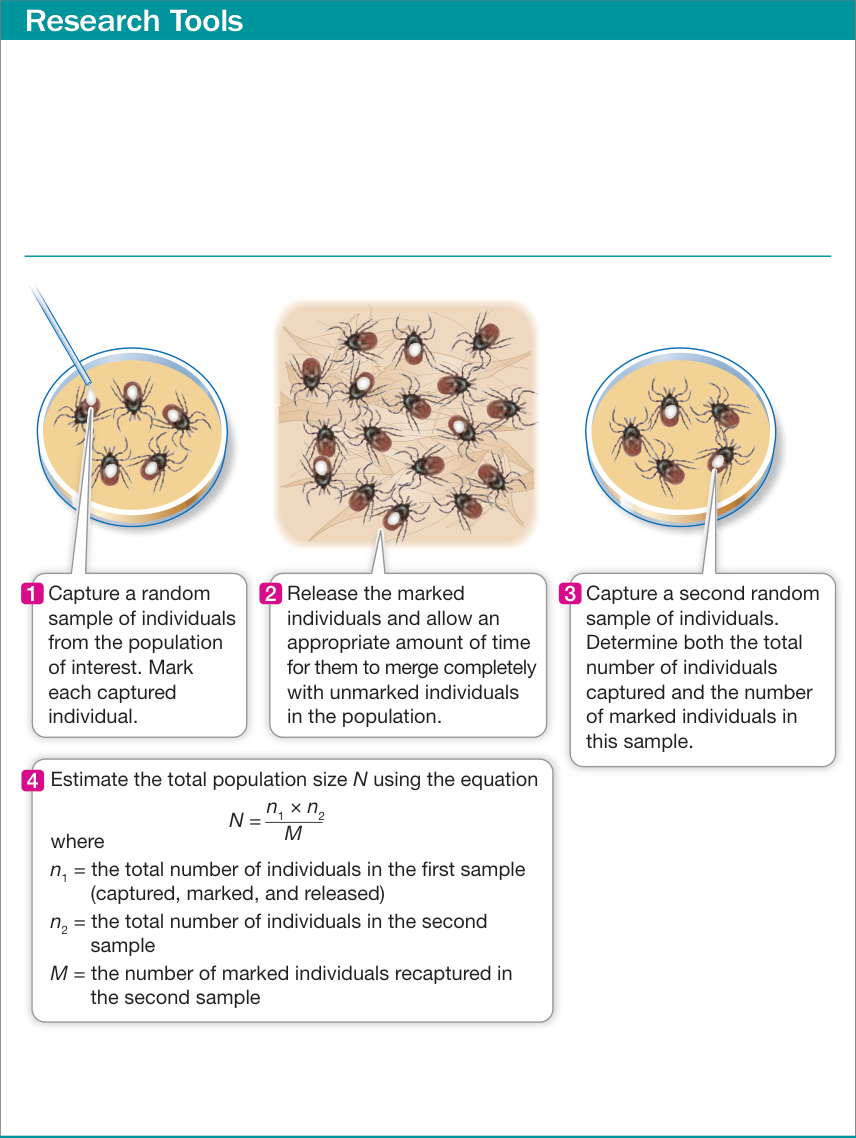
Figure 53.5A The Mark–Recapture Method The method described here is used to estimate animal population sizes for highly mobile species (such as Ixodes scapularis, the black-legged tick). Once a sampling area has been determined, investigators capture, mark, and then release the animals back into the population. The proportion of marked individuals recaptured in a second sample is assumed to be the same as the proportion of the total individuals in that sample to the population size within the area.
called a quadrat or along a transect—a line drawn across an area within the range of the population (often designated by a tape measure marked at regular intervals). By making repeated counts with either of these methods, investigators can use these surveys to make reasonably good estimates of the size of a population.
Counting mobile organisms is more difficult because individuals move into and out of sampling areas, as you saw in the humpback whale example. In such cases, investigators may use the mark–recapture method (Figure 53.5). They begin by capturing, marking, and then releasing a number of individuals. Later, after the marked individuals have had time to mix with unmarked individuals in the population (but before enough time has elapsed for births, deaths, and individual movement to affect the population size significantly), another sample of individuals is captured. This sample is then used to obtain an estimate of the total size of the population in the sampling area. The extrapolation is achieved by applying the equation described in Figure 53.5A, which assumes that the proportion of marked individuals in the second sample (i.e., individuals that were captured and marked in the first sample) is about the same as the proportion of individuals in the sampling area that were captured in the first sample.
More recently, ecologists have used DNA analysis to determine how many unique individuals might be contained within a population. In some cases, instead of capturing individuals and collecting DNA, ecologists collect the next best thing—tissues, fur, or feces left behind by animals in their natural habitat to be analyzed for DNA signatures. In a novel twist on sample collection, some ecologists have even trained dogs to locate feces of some hard-to-find species such as orca whales (Orcinus orca). With enough samples, the extent and size of populations can then be determined for species that are hard to survey in the wild.
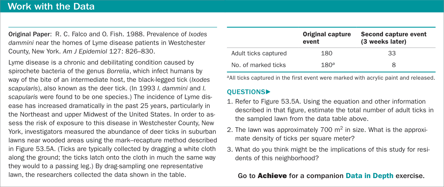
Figure 53.5B Monitoring Tick Populations
Recap and Assess
Species are divided into groups of individuals, or populations, that can vary spatially across their geographic range. All populations change in size and spatial extent due to the physical environment, biological interactions, and dispersal. Ecologists use a variety of approaches to estimate population sizes, including full censuses, surveys using quadrats or transects, mark-recapture methods, and DNA analyses.
- Refer to Figure 53.4. Draw a diagram showing which populations of humback whales interact on their summer feeding grounds. Do you think all five populations make up one metapopulation during the summer? Explain.
- Refer to Figure 53.2. What type of species interaction appears to have caused the aphid population to fluctuate in size? What type of species interaction keeps the population size from fluctuating?
- A researcher wants to determine how many leopard frog tadpoles are present in a pond in the spring. Later, after the tadpoles have metamorphosed, she wants to compare this number with the size of the frog population. What method should the researcher use to determine the population sizes? Explain your answer.
Quantifying population sizes in space and time provides valuable information on the dynamics of a species, but those observations alone cannot explain how, when, and why populations change in size. In order to understand and predict population sizes through time, ecologists characterize population growth, or the change in population size over time, using quantitative methods.
Population Growth Describes the Change in Population Size over Time
Population Growth Describes the Change in Population Size over Time
Learning Objectives
53.2.1 Devise equations for exponential and logistic population growth, and explain each of the terms of the equation.
53.2.2 Use exponential and logistic population growth equations to predict population size at some time in the future.
53.2.3 Distinguish between density-dependent and density-independent factors in population growth.
53.2.4 Interpret a life table, and explain and calculate the type of information it can provide about a population.
It is clear from Key Concept 53.1 that populations are constantly changing in size. Population growth describes the change in population size over time. For example, you read that North Pacific humback whales experienced dramatic declines in population size from commercial whaling, but when hunting was banned, the populations rebounded from 1,400 whales in 1966 to nearly 20,000 in 2006. Measuring how a population changes over time requires following its demography: births, deaths, immigration, and emigration.
Births increase and deaths decrease population size over time
Over any given interval of time, the size of a population increases by the number of individuals added to the population by births and by immigration (the movement of individuals into the population from elsewhere) and decreases by the number of individuals lost from the population by deaths and by emigration (individuals leaving the population to go elsewhere). This relationship is expressed mathematically as
where = the population size at time , = the population size at time 0, = the number of individuals born between time 0 and time , = the number that died between time 0 and time , = the number that immigrated between time 0 and time , and = the number that emigrated between time 0 and time .
As you saw earlier, population size rarely remains the same but instead changes over time. We can use Equation 53.1 to estimate how population size changes over the interval of time 0 to and get a population growth rate, or the rate of change in population size over time. This can be expressed mathematically as
or the change in () for the time interval 0 to
To understand population growth rate from births and deaths alone, ecologists often assume a “closed system” that does not include immigration and emigration. This simplifies the equation to
The change in population size can then be calculated if one knows the number of births () and deaths () that have occurred over a given period of time. The birth and death numbers will naturally depend on the size of the population and the time interval considered. As a result we need to convert and into rates that will allow us to estimate population growth for any change in population size over time. Therefore we can further express and as
where is the product of the per capita birth rate () (i.e., the number of births per individual per unit of time) and (population size at time 0). Likewise, the death rate can be calculated as
where is the product of the per capita death rate () (i.e., the number of deaths per individual per unit of time) and (population size at time 0).
The term “per capita” literally translates to “per head” and is meant to indicate births and deaths per individual in the population. The change in the total number of births and deaths can then be calculated by multiplying the per capita birth and death rates by the population size at . Here’s what that looks like mathematically:
The difference between the per capita birth and death rate () is the per capita growth rate (). Substituting for , we get
This simple model reflects why populations change in size. A population will increase in size if the per capita birth rate exceeds its per capita death rate; that is, if , then . Likewise, the population will decline in size if , or . If , then , and the population will not change in size.
Ecologists use differential calculus to express the change in population size () over very short, instantaneous periods of time (). In this way, they are assuming that population growth is continuous, meaning the time interval is infinitely small and the growth curve will be smooth. This is expressed by
Once we have a value for , and we know population size, we can use it to characterize patterns of growth in populations through time. One pattern of growth that occurs when populations are not limited by resources is exponential growth, which we discuss next.
All populations have the potential for exponential growth
You know from Equation 53.4 that a population will grow, over some time period, as long as the per capita growth rate, , is greater than zero (that is, when ). During this time period, the population will add a number of individuals that is times its initial size. As the number of individuals in a population () increases, the number of new individuals added per unit of time accelerates—that is, increases—even though the per capita growth rate () remains constant (Figure 53.6). This multiplicative pattern is known as exponential growth. It is also clear from Figure 53.6 that the value of can make a big difference in the rate of growth of the population—a population with will have a much faster rate of growth than a population with , even though both populations will display an exponential growth pattern.
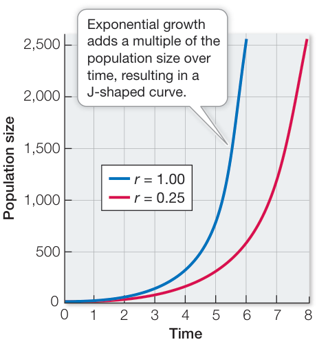
Figure 53.6 Exponential Population Growth Rate Exponential population growth occurs when the size of a population changes by a constant proportion over time. This graph compares the exponential growth of two populations that vary in their values of . Q: Which curve, blue or red, has the faster population growth rate?
Equation 53.4 gives us the exponential growth of a population, but it does not allow us to predict the size of a population at a later time. Using calculus, we can integrate Equation 53.4 and get
where is the population size at time , is the population size at time 0, is a constant, the base of the natural log (), is the per capita growth rate, and is the time interval between time 0 and time . Knowing the starting population size and the per capita growth rate, we can use Equation 53.5 to forecast the population size at some later time, assuming exponential growth. This is similar to the equation that banks use to calculate compound interest on a loan.
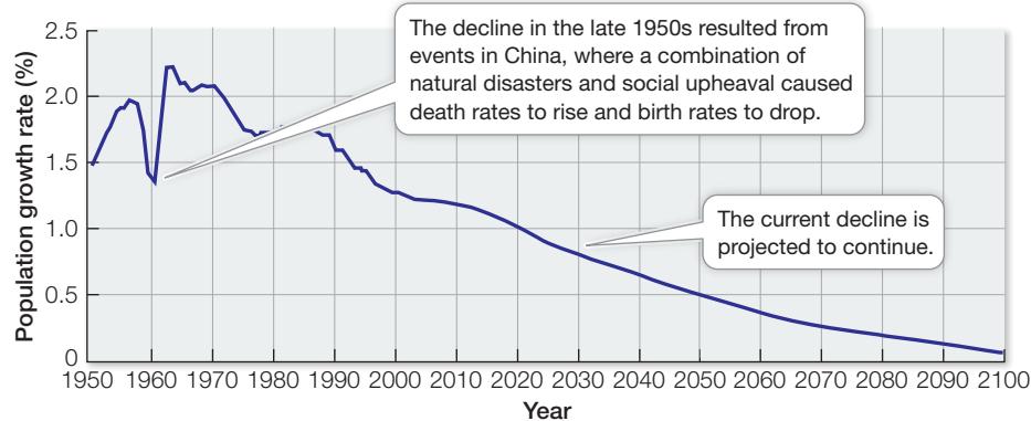
One application of projecting population sizes into the future comes in the form of predicting human population growth. The human population increased relatively slowly until 1825, when it was 1 billion, and now stands at 7.7 billion (Figure 53.7). United Nations data show that world population growth rates have fallen from a high of 2.30%
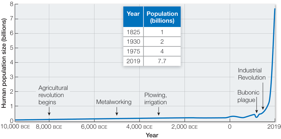
Figure 53.7 Explosive Growth of the Human Population Human population growth was relatively slow until 1825, but advances in technology since then have allowed it to grow at an exponential rate. (Based on estimates by the History Database of the Global Environment (HYDE) and the United Nations. Visualization from OurWorldinData.org. CC BY-SA 4.0/Max Roser. Retrieved from: https://ourworldindata.org/world-population-growth.)
Investigating Life: Will the Global Human Population Growth Rate Decline?
Experiment
Original Paper: United Nations, Department of Economic and Social Affairs, Population Division. 2019. World Population Prospects 2019: Highlights (ST/ESA/SER.A/423).
Understanding the demographic changes in human populations over the coming years is critical in anticipating and planning for such challenges as food production, energy and water consumption, emerging diseases, and climate change facing our planet. The 2019 revision of World Population Prospects is the U.N.’s 26th round of official population estimates and projections. It builds on the previous reports by incorporating results from the most up-to-date national population censuses as well as findings from recent demographic and health surveys that have been carried out around the world.
HYPOTHESIS World population growth rates have declined since 1950 and will continue to decline in the next century.
METHOD►
- Census and demographic survey data on survivorship, fertility, and international migration were gathered for 201 countries over the period 1950 to 2019.
- The demographic data were used to establish parameters for life tables (similar to Table 53.1) in order to determine human population growth rates from 1950 to 2019.
- To project the change in population growth rate values up to 2100, demographic data were used to make assumptions on future trends in human survivorship, fertility, and international migration. Because the future is uncertain, several different projections were produced to understand their possible variability and arrive at a “best estimate” of the change in population growth.
RESULTS Population growth rates fluctuated after 1950 but dropped from a high of 2.30% in the early 1960s to 1.10% in 2019. Projections indicate that human population growth rates will continue to decline to 0.50% in 2050 and to 0.10% in 2100. Note that the percent population growth rate is equivalent to .
CONCLUSION Population growth rates have dropped substantially in the last 69 years and are projected to continue this trend into 2100.
Data from U.S. Census Bureau, International Data Base, 2018; United Nations, Department of Economic and Social Affairs, Population Division (2019). World Population Prospects 2019: Highlights (ST/ESA/SER.A/423). Graph after Max Roser et al. 2019. World Population Growth. Published online at OurWorldInData.org. CC BY-SA 4.0
(note that the percent population growth rate is ) in the early 1960s to 1.10% today (Investigating Life: Will the Global Human Population Growth Rate Decline?). Projections indicate that human population growth rates will continue to decline to 0.50% in 2050 and to 0.10% in 2100, leading to a “best estimate” population size of 9.7 billion by 2050 and 11 billion by 2100. These projections in human population size beg the question: will world resources be able to sustain such large populations into the future? Is 11 billion above the maximum number of humans that can be supported sustainably on Earth? We will consider these questions at the end of the chapter.
Some populations may grow at rates close to their maximum, depending on the circumstances. During the 39 years following the ban on commercial whaling, North Pacific humpback whale populations grew exponentially at a rate of 5%–7% per year. Since the whales were released from hunting, they have had ample habitat, abundant food, and no predators, so there appeared to be little limiting their population growth at that time. However, changes in ocean conditions and thus food resources, entanglement in fishing gear, ship strikes, whale-watching harassment, and harvesting for scientific purposes all pose potential threats to humpback whale population recovery. In addition, there will always be some limit to the population sizes whales can attain, given intraspecific competition for food resources and breeding areas.
Work with the Data
Here you will use the population growth rate from above to project the human population size on Earth in the future.
QUESTIONS►
- Using Equation 53.5, the population size in 2019 (7.7 billion), and the population growth rate for 2019 (1.10%), estimate what the world’s population size will be in 2100.
- Projections indicate that if the human population growth rate declines to 0.50% in 2050, the population size will be 9.1 billion by 2050 and 10 billion by 2080. Using the projected population size and growth rate in 2080, project the human population size in 2100.
- Suppose the carrying capacity of Earth is 12 billion people. Using Equation 53.7, project the human population size in 2100, given the 2019 data and 2080 data.
- Given your calculations in Questions 1, 2, and 3, which parameter (population growth rate or carrying capacity) is projected to most reduce population size by 2100?
We will turn next to what happens to population growth when limiting resources affect the number of births and deaths within a population.
Logistic growth occurs as a population approaches its carrying capacity
What would happen if all the offspring produced by a population survived and reproduced? The prospects are alarming. In 1911 L. O. Howard, then chief entomologist of the U.S. Department of Agriculture, estimated that if all the offspring of the common house fly (Musca domestica) were to survive, a pair of flies beginning to reproduce on April 15 would produce a population of 5,598,720,000,000 adults by September 10 of the same year. Given such amazing reproductive capacities, it is clear that forces exist to limit the growth of fly populations (and populations of every other organism).
No real population can maintain exponential growth for long periods of time. As a population increases in density, the resources it requires—such as food, nest sites, and shelter—become depleted, causing birth rates to drop and death rates to rise. In other words, birth rates and death rates are dependent on the density of the population. Populations may initially grow rapidly when the population is small, but as populations increase in size, density-dependent birth and death rates cause to decline toward zero, a pattern of population growth called logistic growth. Eventually when , the population stops changing in size because births equal deaths. Thus instead of continuing to increase exponentially, population growth slows down and the population eventually levels off at some size known as the carrying capacity, or (Figure 53.8). can be thought of as the number of individuals that any particular environment can sustain indefinitely. If the number of individuals in the population exceeds , then will be negative until population size reaches once again. Likewise, if the number of individuals falls below , then will be positive until population size reaches .
To model logistic growth, the exponential growth equation is modified by adding a term, , which represents the fraction of the carrying capacity () that is available for population growth. As long as the population size is less than the carrying capacity (i.e., ), only a fraction of the available resources are being used. As the population size approaches the carrying capacity, however, the fraction of resources available for any new individual becomes smaller. The logistic growth equation is simply the exponential growth rate multiplied by to get
Population growth should stop when because at that point, , so , and thus and the population will remain at a constant size.
Just as you saw with Equation 53.5, we can integrate Equation 53.6 to allow us to predict the population size at some later time, assuming logistic growth. When we do this we get
where is the population size at time , is the population size at time 0, is carrying capacity, is a constant, the base of the natural log (), is per capita growth rate, and is the time interval between time 0 and time . In this case, knowing the starting population size, the per capita growth rate, and the carrying capacity of the population, we can use Equation 53.7 to forecast population size at some later time, assuming logistic growth.
Factors limiting population growth can be density-dependent or density-independent
As you just saw, the density of a population can have large effects on population growth and ultimately the size of a population through time. Density-dependent factors can include:
- Limiting resources. As a population increases, it depletes its resources as a result of intraspecific competition.
- Predators may be attracted to areas with high densities of their prey, allowing them to capture a larger proportion of individuals and causing the death rate of the prey population to rise.
- Pathogens may spread more easily in dense populations than in populations with fewer individuals, resulting in a rise in the death rate.
It is important to note that density does not always cause a decline in population growth. Some populations grow better, albeit up to some limit, when population densities are higher rather than lower; this is known as the Allee effect (named after the ecologist W. C. Allee, who first described it). Sometimes individuals survive better in a group than on their own, as you saw with the predator avoidance strategies used by wood-pigeons and ground squirrels living within groups (see Figure 51.21).
Moreover, not all factors that change population size act in a density-dependent manner. A period of extreme cold, or an exceptionally strong hurricane, may kill a large number of individuals in a population regardless of the population’s density; such an event is density-independent and may be a significant factor in depressing growth and keeping populations from reaching their carrying capacity.
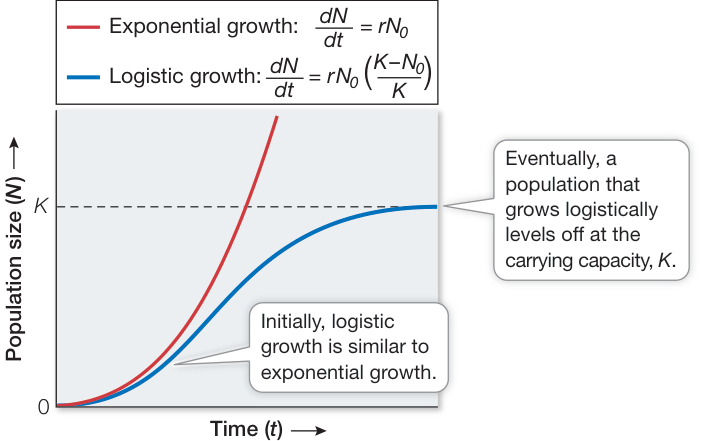
Figure 53.8 Population Growth Models: Exponential versus Logistic Growth Exponential population growth (red J-shaped curve) is much faster than logistic population growth (blue S-shaped curve), which is limited by the density or carrying capacity of the population.
Life tables keep track of demographic events
Up to this point we have assumed that individuals within a population do not vary in their birth and death rates. This is a big assumption given that we know real populations are made up of individuals of different ages, sizes, and sexes, which vary in their capacity to reproduce or survive. For example, a newborn whale or human cannot reproduce immediately, and must mature to reproductive age. Likewise, the likelihood of death will vary depending on the age of the individual. Ecologists use a form of accounting, known as a life table, to keep track of how demography will affect the growth rate of the population. Life tables summarize how survival and reproductive rates vary with the age, size, or sex of the individuals within a population. These summaries can then be used to predict future population trends and develop strategies for managing populations of commercial or ecological value. They are also used by life insurance companies to determine how much to charge people of different ages for insurance policies.
Let’s consider an example of a life table from the literature. Table 53.1 shows a cohort life table using data from the acorn barnacle Balanus glandula on the shorelines of Scotland. A cohort life table uses a cohort—a group of individuals born within the same time frame—from the larger population to estimate growth rate. The two columns on the left show the number of individuals surviving and the number of offspring produced at different ages () through time. As the individuals within the cohort die, decreases from 1 million barnacles to only 2 barnacles after 8 years. The proportion of individuals that survive, known as survivorship (), can be calculated by simply dividing by , the number of barnacles originally born into the cohort (represented by age 0). In addition, we can calculate the fecundity (), or the mean number of barnacle offspring produced per surviving adult barnacle per age class, by dividing the total number of offspring ( offspring) by the number of individuals () that produce those offspring. Multiplying survivorship () by fecundity () gives us the number of offspring produced for individuals within a particular age class within the population. The sum of these values for all the age classes gives us the net reproductive rate, , which is simply the mean number of offspring produced per individual in the cohort, adjusted for survival:
If is greater than 1.0, there is a net increase in offspring produced each generation, and assuming the birth and death rates do not change over time, the population should increase exponentially. If is less than 1.0, and individuals are not replaced as they die, the population declines eventually to extinction. If is 1.0, then the births and deaths balance out and the population will not change in size.
We can use to estimate the per capita growth rate, , of a cohort by scaling to account for the generation time of the cohort. The generation time, , is the average age of the parents of all the offspring produced within the cohort (see Table 53.1 for equation). To estimate , we simply divide the natural log () of by and get
Cohort life tables follow individuals from birth to death as a function of calendar year or life stage (e.g., eggs, larvae, pupae, and adults in insects). This is relatively easy to do if the organisms are easily followed—for example, if they are sessile and short-lived as we saw in the barnacle example. For organisms that are harder to track, a static life table can be constructed by sampling a population at a single slice of time. Here the numbers of individuals and their reproduction for different age classes are recorded at one time and used in a similar way as those data in Table 53.1 to calculate the net reproductive rate and per capita growth rate of the population.
The construction of life tables has allowed ecologists to observe common life history patterns, reflecting common solutions to ecological challenges, across a tremendous diversity of organisms. For example, the number of individuals surviving through each life stage (survivorship, ) can be taken from a life table and plotted graphically to construct a survivorship curve. Typically, a survivorship curve is constructed for a hypothetical cohort, usually of 1,000 individuals, by plotting the numbers of individuals expected to survive to reach each age category on a logarithmic scale.
Table 53.1 Cohort Life Table for the Barnacle Balanus glandulaa
| Age () | Number of individuals () | Number of offspring ( offspring) | Survivorship () | Fecundity () | ||
|---|---|---|---|---|---|---|
| 0 | 1,000,000 | 0 | 1 | 0 | 0 | 0 |
| 1 | 62 | 285,200 | 0.000062 | 4,600 | 0.285 | 0.285 |
| 2 | 34 | 295,800 | 0.000034 | 8,700 | 0.296 | 0.592 |
| 3 | 20 | 232,000 | 0.000020 | 11,600 | 0.232 | 0.696 |
| 4 | 15 | 190,500 | 0.000015 | 12,700 | 0.191 | 0.764 |
| 5 | 11 | 139,700 | 0.000011 | 12,700 | 0.140 | 0.700 |
| 6 | 6 | 76,200 | 0.000006 | 12,700 | 0.076 | 0.456 |
| 7 | 2 | 25,400 | 0.000002 | 12,700 | 0.025 | 0.175 |
| 8 | 2 | 25,400 | 0.000002 | 12,700 | 0.025 | 0.200 |
1 To estimate the per capita growth rate, , sum all by values to get the net reproductive rate, .
2 Then, sum all by by values and divide by to get the generation time, .
3 Finally, divide the natural log of by to get the intrinsic rate of increase, .
Source: Data from J. H. Connell. 1970. Ecol Monogr, Ecological Society of America 40: 49–78.
aThe life history of barnacles involves releasing larvae into the water column, where they feed and undergo a series of larval stages. Eventually they settle back on the rock and metamorphose into a juvenile barnacle, which grows into a reproductive adult.
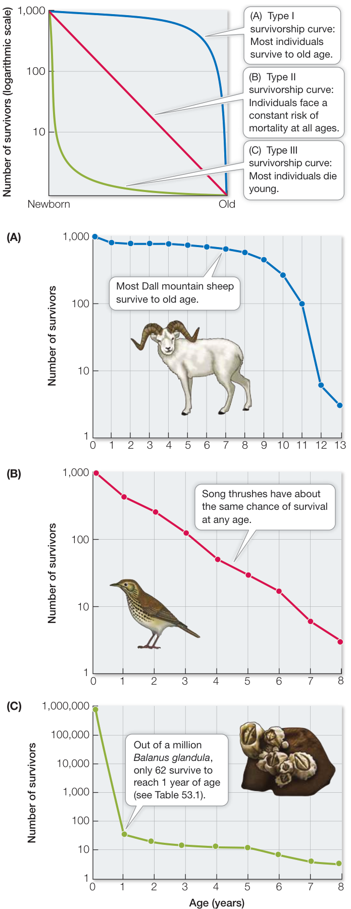
Figure 53.9 Survivorship Curves Ecologists recognize three general types of survivorship curves. Notice that the number of survivors has been plotted on a logarithmic scale. Three species provide real-world examples of the three types of life histories. (A, B after E. S. Deevey. 1947. Q Rev Biol 22: 283–314; C after J. H. Connell. 1970. Ecol Monogr, Ecological Society of America 40: 49–78.)
Q: What type of survivorship curve do humans have?
Survivorship curves tend to take one of three general shapes:
- Species with type I survivorship curves experience high overall survivorship through adulthood but steep declines late in life (the curve is concave) (Figure 53.9A). Species with this type of survivorship curve (humans, elephants, whales, and many other large mammals) typically have low reproduction rates but provide parental care to their offspring, which reduces the risk of death in early stages of development.
- Species with type II survivorship curves face a constant risk of mortality at all ages (the curve is linear) (Figure 53.9B). Many birds, fishes, and plants display this pattern.
- Species with type III survivorship curves experience low survivorship early in life and higher survivorship once they reach maturity (the curve is convex) (Figure 53.9C). Species with this type of survivorship curve (most insects; marine invertebrates, including the barnacle in Table 53.1; and annual plants) tend to produce many offspring but provide little or no parental care.
Species survivorship curves help us classify how mortality plays out in populations over time, but many species have patterns of survivorship somewhere in between these extremes. For example, some organisms show a “stair-stepped” curve, with bouts of mortality during vulnerable periods of their life, followed by periods of relatively low mortality.
Recap and Assess
Population growth is the change in population size over time, as reflected by the number of births, deaths, and migrants in and out of the population. Exponential (multiplicative) growth occurs when the per capita growth rate, , is constant over time. Logistic growth occurs in an environment in which resources are limited and a population reaches its carrying capacity, . Factors limiting population growth can be density-dependent (e.g., competition for food or space) or density-independent (e.g., environmental conditions). Life tables summarize how survival and fecundity vary with the age, size, or sex of the individuals in a population, and predict how these demographic events affect population growth.
- Write an equation that describes how births, deaths, immigration, and emigration affect population size. Define each variable.
- Suppose you are asked to predict what the population size of an
endangered bird will be in 2040.
- Complete the following cohort life table, and calculate the , , and of this cohort.
| Year | Age (x) | Number of female birds () | Number of female offspring () | Survivorship () | Fecundity () | Net reproductive rate () | Generation time () |
|---|---|---|---|---|---|---|---|
| 2017 | 0 | 100 | 0 | ||||
| 2018 | 1 | 50 | 75 | ||||
| 2019 | 2 | 40 | 80 | ||||
| 2020 | 3 | 30 | 60 |
We know as humans that individuals vary widely in when they mature, when and how many children they have, and when they die. This lifetime pattern of growth, reproduction, and survival is known as an individual’s life history. In addition to the variation we see in life history patterns at the individual level, all species have a common life history strategy that helps define the average timing and nature of important life history events (Figure 53.10). Life history strategies are shaped by the way individuals within and among species allocate resources to growth, reproduction, and survival based on genetic and environmental factors. For example, in the case of humans today, the average age of puberty is 11 years, the average woman has one child at a time (except in the rare cases of multiple births), and the average life span is 70 years. These life history statistics are a product of the environmental and genetic constraints placed on humans in the twenty-first century. But they also belie the fact that human life history traits have changed dramatically from historical times and vary widely among populations around the world. Thus as you will see, life history patterns not only vary within and among species but also through time.
- Calculate what the population size, , of this cohort will be in 2040, assuming exponential population growth and .
- To add more realism to these calculations, suppose that (carrying capacity) = 300 for this cohort. What will the population size be, assuming logistic growth, in 2040?
- Plot the number of birds surviving with age for the cohort in Question 2. What type of survivorship curve does this cohort have?
- Describe some density-dependent and density-independent factors that could control the population growth of the bird cohort in Question 2.
Life tables reflect the ways in which organisms partition their time and energy among growth, maintenance, and reproduction. Comparisons across individuals, populations, and species reveal different patterns of partitioning, which allow organisms to cope with different environmental challenges. Let’s move on to discuss how life history traits arise and the types of strategies organisms employ.
Life history strategies can vary at species and population levels
Life history strategies can vary among species, even for species that are taxonomically closely related, as a consequence of environmental differences. For example, on Mount Kenya two species of unusual plants in the genus Lobelia live in different types of habitats (Figure 53.11). One species, Lobelia telekii, lives on the dry rocky slopes of the mountain, where it reproduces only once (a strategy called semelparity), produces vast numbers of small seeds, and has a short life span. In the moist valley bottoms, another species, Lobelia keniensis, reproduces more than once (a strategy called iteroparity), produces fewer but larger seeds per reproductive event, and lives longer. Semelparity is typical of organisms whose probability of dying remains high even when they reach adulthood; it is seen in
Life History Is the Lifetime Pattern of Growth, Reproduction, and Survival
Learning Objectives
- 53.3.1 Distinguish between the relative contributions of environment and genetics to life history traits in specific situations.
- 53.3.2 Describe how and why life history trade-offs might arise in a species or population.
- 53.3.3 Distinguish between r-strategists and K-strategists, and identify specific situations in which evolution might favor one strategy over the other.
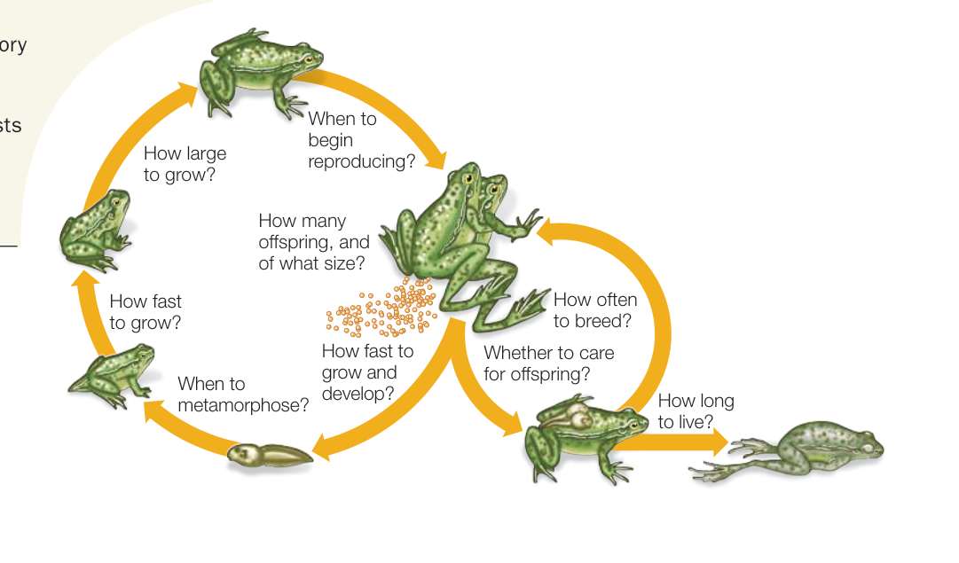
Figure 53.10 A Life History Strategy The timing and nature of life history events shape the overall life cycle of an organism. The life history strategy of this frog species reflects how environmental and genetic factors affect strategies to optimize growth, reproduction, and survival.
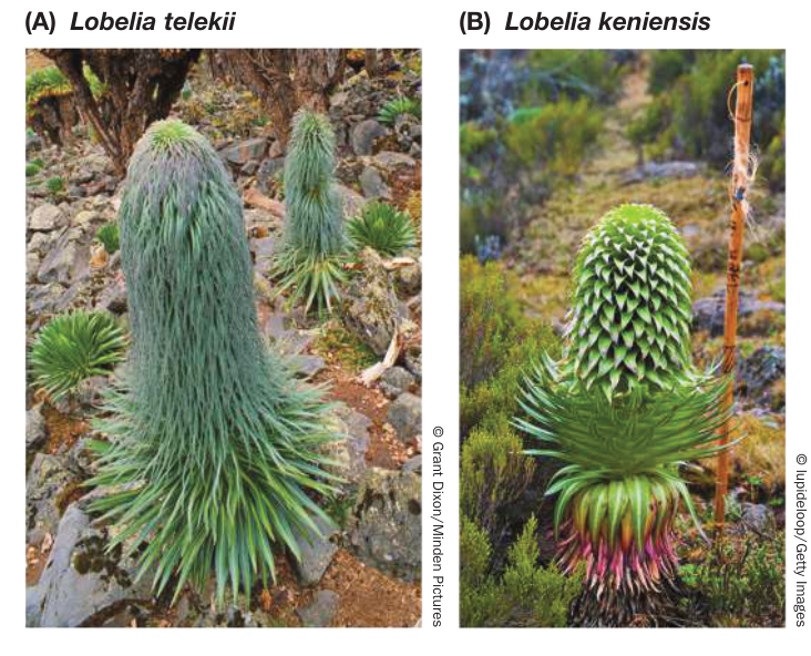
Figure 53.11 Related Species with Vastly Different Life History Strategies On Mount Kenya, Africa, (A) Lobelia telekii lives on the dry rocky slopes of the mountain, where it reproduces once (is semelparous), produces many seeds, and has a short life span. In the moist valley bottoms, (B) Lobelia keniensis reproduces multiple times (is iteroparous), produces fewer but larger seeds, and lives longer.
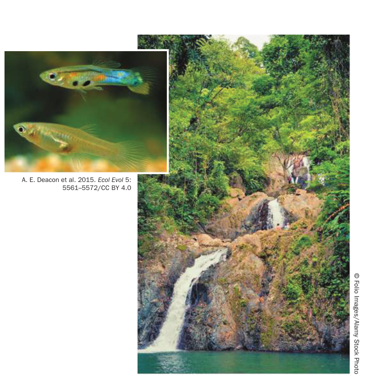
Figure 53.12 Predation Affects the Life History of Guppies In Trinidad, populations of guppies (Poecilia reticulata) from high-predation stream sites below the falls matured earlier, reproduced more frequently, and produced more offspring per brood compared with guppies from low-predation stream sites above the falls, no matter how many resources the guppies were given. Q: Are the life history strategies of the two guppy populations, one from high-predation streams and the other from low-predation streams, likely genetically determined? Why?
some fishes, many insects, and all annual plants. In contrast, iteroparity is typical of organisms with long life spans. For example, because environmental conditions within the nests of social insects such as honey bees and ants are remarkably stable, iteroparity is the rule among these species; some queens live 10 years or longer and reproduce over their entire adult lives.
Life history strategies can also vary within species at the population level. For example, some populations of guppies (Poecilia reticulata) in Trinidad live in streams where they are attacked and eaten by larger fishes (Figure 53.12). But some streams have waterfalls that predatory fishes are unable to negotiate. Guppies that live in the predator-free areas upstream from those waterfalls have lower death rates compared with guppies below the falls. To see whether the risk of being eaten by a predator influenced the life history strategies of these guppies, David Reznick and his colleagues collected guppies from high-predation and low-predation sites and raised them in the laboratory. Some guppies from each group were provided with plentiful food, and others with limited food, to simulate the variation the fish would typically encounter in their home streams. In the laboratory, where no predators were present, guppies from high-predation sites matured earlier, reproduced more frequently, and produced more offspring in each brood than did guppies from low-predation sites, no matter how much food the guppies received. The investigators concluded that predation had genetically selected for early and frequent reproduction in the guppies living below the falls.
Perhaps the best-studied example of how life history traits can vary not only among populations, but also among individuals, is the case of human life span. Human life span varies widely around the world and between the sexes (Figure 53.13). Today, humans live on average to 87 years in Japan, Hong Kong, and many European countries, and to 35–50 years in some African countries (e.g., Sierra Leone, Democratic Republic of the Congo, and Somalia) where HIV infection, famine, and war are common. In the United States, average life span is 80 years, with women outliving men by 5 years. Research has shown that the factors contributing to lower life expectancy rates in men include higher rates of homicide, accidental death, and parasitic and infectious diseases.
For the most part, the large variability in life span we see in humans can be attributed to environmental factors. If you lived during the Bronze Age, your life expectancy was 28 years, and it was not much better even in the early nineteenth century (about 35 years). Reduction in infant mortality has accounted for most of the increase in life expectancy, but since the end of the 1950s the mortality rate of those older than 80 years has decreased by 1.5% each year. Much of the increase in life expectancy that we enjoy today is the result of modern advances in human health and nutrition, which begs the question: is there a limit to human life expectancy? One study, which plotted human life-span data over time, shows a remarkable linear relationship with no leveling off yet, which could indicate an upper limit (Figure 53.14). In fact, because life span has increased by 2.5 years every decade for the last 150 years, one possible scenario is that 60 years from now the average person’s life span will reach 100 years! While some limit on human life span is almost certain, these predictions suggest that human life expectancy is a highly flexible life history trait indeed.
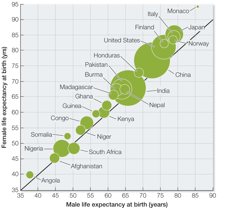
Figure 53.13 Human Life Expectancy around the World Comparison of recent male and female life expectancy at birth for a variety of countries. The solid black line corresponds to equal female and male life expectancy. The sizes of the bubbles are linearly proportional to the population of the country. (Data from The World Factbook 2016-17. Washington, DC: Central Intelligence Agency, 2016. https://www.cia.gov/library/publications/the-world-factbook/index.html)
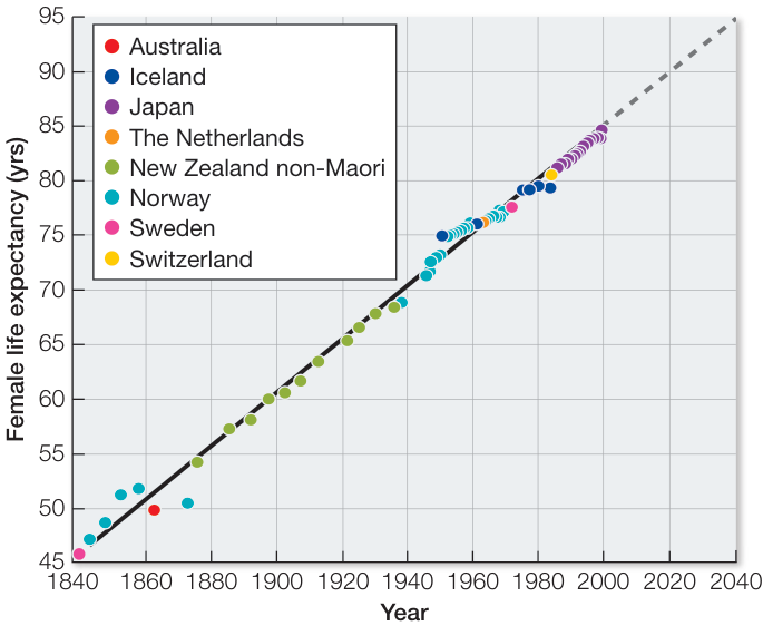
Figure 53.14 Human Life Expectancy—Past, Present, and Future Recorded human female life expectancy from 1840 to the present. The linear trend in life expectancy is depicted by the bold line, and the extrapolated trend by the dashed gray line. Based on the trend, in 2040 the average woman might have a life span of 95 years. (After J. Oeppen and J. W. Vaupel. 2002. Science 296: 1029–1031.) Q: Compare the differences in female life expectancy between 1840–1940 and 1940–2040. Is the rate of change in life expectancy predicted to increase?
Life history strategies arise from constraints on growth, reproduction, and survival
As it should be clear by now, the fitness of a population or species is highly dependent on its life history strategy in relationship to its surrounding environment. Thus it makes sense that genes that maximize growth, reproduction, and survival would be favored by natural selection, resulting in an optimal life history strategy for that species or population. However, there are constraints on optimality, resulting in trade-offs in life history traits that put limits on the possible life history outcomes for species.
Connect the Concepts Key Concept 21.5 describes how constraints on optimality include genetic variation for evolution to act on, as well as the mediating effects of the physical and biological environment.
Trade-offs include allocation of resources to such traits as growth versus reproduction or number of offspring versus their body size. Energy devoted to one life history trait can reduce the amount available for others. For example, the growth of Douglas fir trees (Pseudotsuga menziesii) measured using annual growth ring size is negatively correlated with cone production. The more cones the tree produces, the narrower the width of the rings, suggesting that the allocation to reproduction takes energy from growth. Another trade-off that can have dramatic consequences for population growth is that of survival and reproduction. An example of this occurs in the giant Pacific octopus (Enteroctopus dofleini), which lives only 3–5 years and dies soon after significant parental investment in its thousands of offspring.
As you have seen, much of the variation in life history traits appears to result from an evolutionary response to environmental variability. Generally, unpredictable environments are associated with greater allocation to reproducing quickly, shorter life spans, and correspondingly high per capita growth rates. Conversely, predictable environments, where organisms must compete for high-quality resources, are associated with lower fecundity, longer life spans, and correspondingly lower per capita growth rates. Species whose life history strategies allow for high population growth rates are called r-strategists, and species whose life history strategies allow them to persist at or near the carrying capacity () of their environment are called K-strategists (Figure 53.15). Keep in mind, however, that these categories are extremes; most species fall along a continuum between these two strategies.
For r-strategists, life is uncertain. Individuals tend to reproduce only once and to produce large numbers of offspring, most of which are expected to die early in life (that is, they have a type III survivorship curve; see Figure 53.9C). They can generally use a wide variety of resources and tolerate a wide range of conditions. K-strategists are adapted to predictable conditions, are long-lived, and reproduce several times; their smaller numbers of offspring have a high probability of surviving to adulthood (that is, they have a type I or II survivorship curve; see Figure 53.9A,B). K-strategists tend to be good at enduring competition for resources, but this sometimes leads to trade-offs in reproduction.
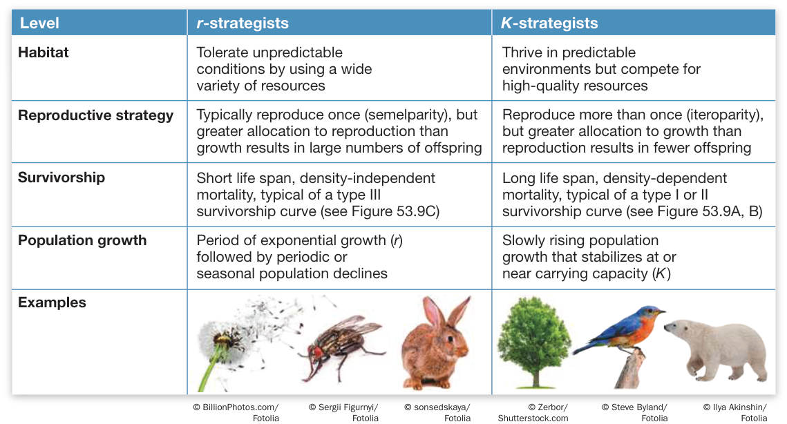
Figure 53.15 Two Life History Strategy Types Species whose life histories are geared to achieve the maximum possible rate of population growth are referred to as r-strategists; those whose population dynamics are bounded by carrying capacity are K-strategists. The life histories of most species fall along a continuum between these two extreme strategies.
That life history trade-offs can evolve is suggested by genetic correlations among suites of life history traits. Such genetic correlations imply either simultaneous selection on two or more life history traits or linkages among the genes that code for those traits. Across Drosophila melanogaster strains, for example, a high per capita rate of growth is correlated with the ability to reproduce under starvation conditions and with the ability to develop on a variety of media in the laboratory—both of which are consistent with the r strategy of tolerating a wide range of resources and conditions.
Connect the Concepts Key Concept 12.4 describes how linked genes occur together on the same chromosome and thus are inherited together.
Recap and Assess
An organism’s life history is characterized by its lifetime pattern of growth, reproduction, and survival. All species have a characteristic life history strategy, which arises from genetic and environmental constraints on life history traits. Two extremes of life history strategies include species with high population growth rates (r-strategists) and species that persist at or near their carrying capacity (K-strategists). Most species fall along a continuum between these two strategies.
- Refer to Figure 53.14.
- Does the change in life expectancy for humans over the past 180 years suggest a genetic or an environmental cause?
- Given your answer, are the large differences in human life span for Japan versus Angola, shown in Figure 53.13, likely the result of genetic or environmental factors? Explain.
- Why are species unable to maximize growth, reproduction, and survival? In other words, why are there life history trade-offs?
- Refer to Figures 53.11 and 53.12. What life history strategy types characterize Lobelia telekii versus L. keniensis? How about guppies in high-predation versus low-predation stream sites?
For millennia, humans have tried to increase populations of desirable or useful species and reduce populations of species they consider undesirable. Such efforts are most successful if they are based on knowledge of how those populations grow and what determines their densities.
Population Biology Can Be Used in Managing and Conserving Populations
Learning Objectives
- 53.4.1 Describe the possible density-dependent population approaches to managing both desirable and undesirable species.
- 53.4.2 Analyze the importance of source and sink populations in a metapopulation in terms of their function in conserving a species from extinction.
If we want to manage other species—that is, to increase or decrease their populations—we need to understand their life histories and population dynamics. We turn now to how populations can be managed to our benefit.
Management plans should take life history strategies into account
Knowing the life history strategy of a species can be helpful in managing populations of commercial value. The black rockfish (Sebastes melanops), an important game fish that lives off the Pacific coast of North America, provides one such example. Rockfish have an indeterminate growth pattern—they continue to grow throughout their lives. As in many other animals, the number of eggs a female rockfish produces is proportional to her size, so larger females produce more eggs than smaller females. In addition, older, larger females are better able to provision the eggs they produce with oil droplets, which provide energy to the newly hatched larvae, giving them a head start in life. Larvae from eggs with larger oil droplets, produced by larger females, grow faster and survive better than do larvae from eggs with smaller oil droplets. These life history traits have important implications for the management of rockfish populations.
Because fishermen prefer to catch big fish, intensive fishing off the Oregon coast from 1996 to 1999 reduced the average age of female rockfish from 9.5 to 6.5 years. Thus the females reproducing in 1999 were, on average, smaller than the females reproducing in 1996. This change decreased the average number of eggs produced by females and reduced the average growth rate of larvae by about 50%. This reduction in reproductive ability was linked to a decrease in the ability of the rockfish population to recover from intensive fishing. Maintaining productive populations of rockfish may require regulating the number or size of fish caught, the fishing season, and/or setting aside no-fishing zones where some females can be protected from fishing and allowed to grow to large sizes.
Management plans should be guided by the principles of population dynamics
If we look at a logistic growth curve (see Figure 53.8), we can see that the number of births tends to be highest when a population is well below its carrying capacity. Therefore if we wish to maximize the number of individuals that can be harvested from a population, we should manage the population so that it is far enough below the carrying capacity to have a high birth rate. Hunting and fishing regulations are established with this objective in mind.
Fishes can, however, be overharvested, as illustrated by the story of the black rockfish. Many fish populations have been greatly reduced because so many individuals were harvested that the few surviving reproductive adults could not maintain the population. For example, Georges Bank, off the northeast coast of North America—a source of cod, haddock, and other prime food fishes—was exploited so heavily during the twentieth century that many fish stocks have been reduced to levels insufficient to support a commercial fishery (Figure 53.16). With fishing restrictions the haddock population has rebounded, but the cod population has not.
Many rapidly reproducing species can recover if overharvesting is stopped, but recovery is more difficult for slowly reproducing species. Just as they did with the humpback whale, twentieth-century whalers hunted the blue whale (Balaenoptera musculus), Earth’s largest animal, nearly to extinction. These whales reproduce very slowly: they live up to 10 years before becoming reproductively mature, produce only one offspring at a time, and have long intervals between births. As opposed to humpback whales, however, blue whale populations have recovered more slowly.
Whether we want to manage the sizes of populations of desirable species for sustainable harvesting or of undesirable species for control purposes, the same principles apply. Biological control is the use of natural enemies (predators, parasites, or pathogens) to reduce the population density of an economically damaging species. In many cases the target species is a pest only because it has been introduced to a new area. Natural enemies used for biological control are often obtained from the native region of the pest species. Biological control became popular in the nineteenth century after an outbreak of cottony-cushion scale (Icerya purchasi), an Australian insect that attacks citrus, appeared in citrus groves in California. A predaceous ladybeetle and a parasitic fly were then introduced from Australia. Within a year of their release, these insects brought the scales under control.
Sometimes, however, introduced natural enemies not only fail to have any effect on the pest they were imported to control but also, freed of their own enemies, become pests themselves. This fact underlies the horror story of the cane toad (Rhinella marina) in Australia. This Central American toad was introduced to control cane beetles attacking Australian sugarcane fields. But Australian cane beetles stay high on the upper stalks of the plants; the toads could not reach that high, and thus had no effect on the beetle population. Unfortunately, they had massive effects on other species.
All stages of the R. marina life cycle are poisonous, and Australian reptiles (including snakes and lizards) and mammals that eat them usually die. With no enemies to limit their population growth, cane toads grow fast and outcompete native amphibian species for resources. The toads have spread from northern Australia down the east coast, where they threaten native frog species by preying on them as well as by competing with them. The Australian government is forced to spend millions of dollars in attempting to reduce their numbers.
Knowledge of metapopulation dynamics helps us conserve species
Ecologists have used information on metapopulation dynamics to conserve endangered species. We know from mathematical models that the risk of extinction for a species can depend on the number and size of its populations within a metapopulation, and on the rates of dispersal among them. In some metapopulations there are source populations, which serve as a net source of individuals for sink populations, which receive more immigrants than they produce. Thus although some individual populations may undergo severe decline as a consequence of natural or human-caused factors, source populations within a metapopulation can serve to rescue them.
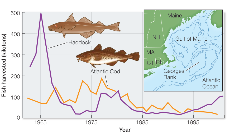
Figure 53.16 Overharvesting Can Reduce Fish Populations Harvests of Atlantic cod (Gadus morhua) and haddock (Melanogrammus aeglefinus) on Georges Bank (map inset) have led to dramatic population declines of both species. Fishing regulations on haddock have allowed its stock to rebound enough to once again support a commercial fishery. (After C. Safina et al. 2005. Science 309: 707–708.)
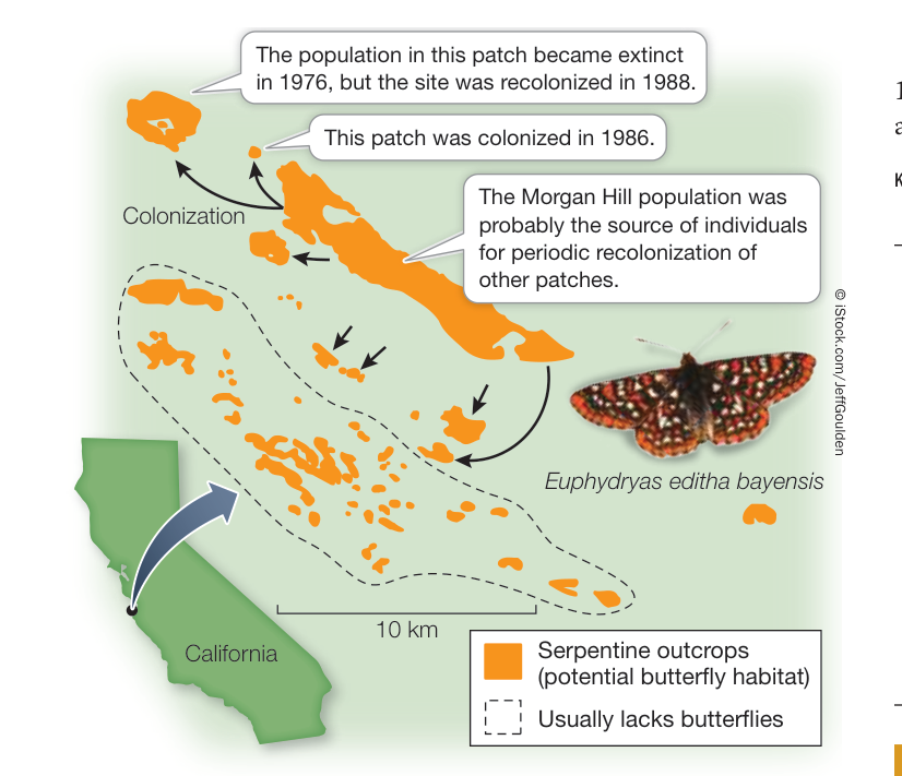
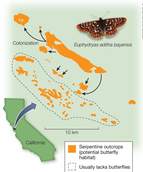
Figure 53.17 A Metapopulation of Checkerspots The San Francisco Bay area metapopulation of Edith’s checkerspot butterfly is divided into several populations confined to patches of suitable habitat on serpentine rock outcrops that contain the food plants of the species. Arrows indicate colonization events. (After S. Harrison et al. 1988. Am Nat 132: 360–382.)
A dramatic example of such metapopulation dynamics is provided by Edith’s checkerspot butterfly (Euphydryas editha bayensis). This endangered subspecies feeds on only two species of annual plants (California plantain [Plantago erecta] and purple owl’s clover [Castilleja exserta]) that are endemic to outcrops of serpentine rock on hills south of San Francisco. In 1960 Paul Ehrlich and his colleagues at Stanford University began studying a population of this butterfly in the nearby Jasper Ridge Biological Preserve and discovered that it was one of several populations within a large, very fragmented metapopulation (Figure 53.17). They followed all the populations over several years and found that they varied in size. During drought years, the butterfly populations declined in size because most of the host plants that the caterpillars relied on died early in the spring, before the caterpillars had a chance to eat them. A severe drought in 1975–1977 led to extinctions of some of the populations. One of the empty habitat patches was repopulated a few years later, most likely by individuals from the largest single population, Morgan Hill, which as late as 1989 contained several hundred thousand butterflies. In 1998, however, the Morgan Hill population, which had historically been the largest in the metapopulation, went extinct. Ehrlich and his colleagues examined 70 years of climate data for the region and concluded that increasing climate variation accounted for the extinction. They also concluded that without a large, stable source population to provide emigrants for recolonization, as the Morgan Hill population did during the
1970s drought, it is unlikely that any of the other populations, which are sink populations, will persist without human intervention.
Recap and Assess
Efforts to manage populations are more likely to be successful if they are based on an understanding of life histories and population and metapopulation dynamics. Biological control is the use of natural enemies to reduce the population density of an economically damaging species. Metapopulations can conserve endangered species if source populations, which supply a source of individuals to sink populations, can rescue those populations from extinction.
- Describe an effective strategy for recovering the population size of a desirable species that has a K-strategist life history.
- Refer to Figure 53.17.
- Describe factors responsible for the metapopulation size of the Edith’s checkerspot butterfly in the San Francisco Bay area.
- Given the 1998 extinction of the Morgan Hill population, what is the likely fate of the metapopulation? Explain your answer.
Investigating Life
QA What is the human population growth projected to be in the next century, and how will that affect population size?
You have seen that this question is highly dependent on the factors that ultimately control the number of births and deaths, or population growth, of humans over time. If the population growth rate projections are correct, there will be roughly 11 billion humans in 2100. Is 11 billion above the carrying capacity of humans? Estimates of the carrying capacity published in 1994 varied tenfold: from less than 3 billion to 44 billion, with the median estimated at 12 billion. As opposed to the carrying capacities of other species, human carrying capacity depends not only on natural constraints important to all species, but also on individual and collective choices concerning the distribution of material goods, the use of technology, and the right to political, economic, and cultural freedoms. The number of people that can live on Earth will depend in part on how many will own cars, eat meat, or have air conditioning. For example, estimates suggest that if the carrying capacity values for the population in the United States were applied worldwide, Earth’s carrying capacity would be limited to 1.2 billion. Compare this with the estimated values for India, where the worldwide carrying capacity could be extrapolated to 14 billion. Given that the current population size on Earth is 7.7 billion, it is clear that the vast majority of humans do not, and will not, experience the quality of life inherent to many in the United States.
Future directions
Some have argued that the number of people that can ultimately live on Earth will depend on the ability of humans to continue to expand their carrying capacity through technological innovations and greater efficiencies in food production and energy generation. These technological innovations will require that we increase food production and natural resource extraction without a heavy reliance on fossil fuels, which have a limited supply and adverse effects on the climate. Ultimately, to believe that no ceiling to human population size is inevitable defies what we know about natural populations.


© Michael Warren/Getty Images
You should be able to relate each summary to the adjacent figures. If you go to this visual summary in Achieve, you can follow links to figures, animations, activities, and simulations that will help you consolidate the material.
Visual Summary
Populations Show Dynamic Variation in Size over Space and Time
- ■ Species are divided into groups of individuals, or populations, that can vary spatially across their geographic range.
- ■ A group of geographically isolated populations linked together by dispersal is known as a metapopulation.
- ■ All populations vary in their dispersion patterns and fluctuate in size over time due to the physical environment, biological interactions, and dispersal.
- ■ Ecologists use a variety of approaches to estimate population sizes, including full censuses, surveys using quadrats or transects, mark-recapture methods, and DNA analysis.
Questions
- What is the difference between a population and a metapopulation?
- What are the three basic dispersion patterns, and what are the main factors that influence them?
- What are some of the ways in which population size and geographic extent of organisms can be measured?
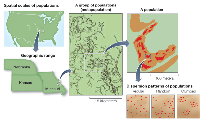
Figure 53.1
Population Growth Describes the Change in Population Size over Time
- ■ Population growth is the change in population size over time, as reflected by the number of births, deaths, and migrants in and out of the population.
- ■ Exponential growth occurs when the rate of change in population size is constant over time. Logistic growth occurs when resources are limited, slowing growth to a population’s maximum size (carrying capacity, or K).
- ■ Factors limiting population growth can be density-dependent when intraspecific competition between individuals affects population growth. Density-independent factors are those that act independently of the population density, such as physical conditions.
- ■ Life tables summarize how survivorship and fecundity vary with the age, size, or sex of individuals within a population, and incorporate how these demographic events affect population growth.
- ■ Species have different types of survivorship curves that reflect mortality patterns over time.
- How does exponential growth differ from logistic growth?
- Describe some density-dependent and density-independent factors that can control population growth.
- How does life table analysis improve the measurements of population growth? Refer to Table 53.1. What type of survivorship curve is characteristic of barnacles?
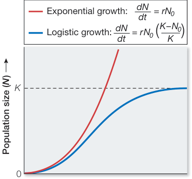
Figure 53.8
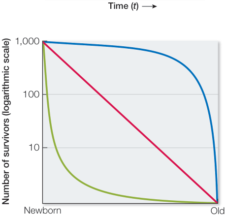
Figure 53.9
Life History Is the Lifetime Pattern of Growth, Reproduction, and Survival
- ■ Life history strategies are characterized by lifetime patterns of growth, reproduction, and survival, and can vary at the species and population levels.
- ■ Life history trade-offs arise from genetic and environmental constraints on optimal growth, reproduction, and survival.
- ■ Extremes in life history strategies of species allow for high growth rates (r-strategists) or for persistence at or near the carrying capacity (K-strategists), but most species fall along a continuum between these two strategies
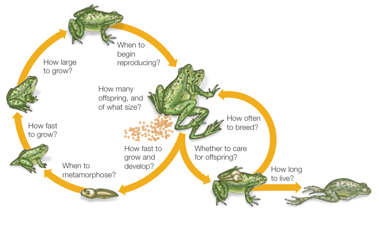
Figure 53.10
Questions
- What are life history traits, and why can they vary among individuals, populations, and species?
- Describe why there are trade-offs in life history strategies.
- How do r-strategists and K-strategists differ?
Population Biology Can Be Used in Managing and Conserving Populations
- ■ Efforts to manage populations are more likely to be successful if they are based on an understanding of life histories and population and metapopulation dynamics.
- ■ Biological control is the use of natural enemies to reduce the population density of an economically damaging species.
- ■ Metapopulations can conserve endangered species if source populations, which serve as a source of individuals to sink populations, can rescue those populations from extinction.
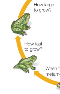
Figure 53.17
Questions
- Describe some ways that population dynamics can be managed for desirable and undesirable species.
- How do source and sink populations within a metapopulation help species avoid extinction?