Chapter 55Communities
Key Concepts
55.1 Communities Are Groups of Interacting Species Occurring Together in Space and Time
55.2 Community Membership Depends on Species Supply, Environmental Conditions, and Species Interactions
55.3 Communities Are Complex Networks of Species Interactions That Vary in Strength and Direction
55.4 Communities Are Always Changing
55.5 Relationships between Species Diversity and Community Function Are Often Positive
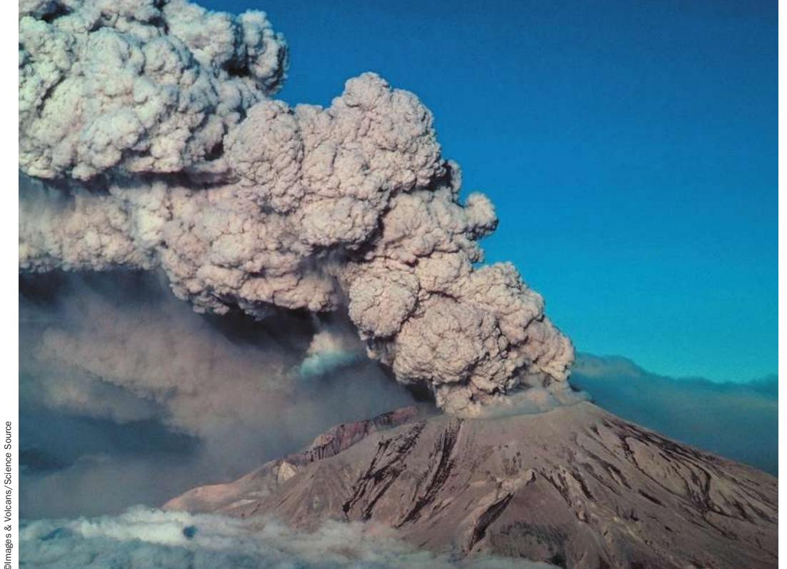
Since its eruption on May 18, 1980, Mount St. Helens has provided a unique opportunity to study community recovery.
©images & Volcans/Science Source
Investigating Life: Rising from the Ashes
When Mount St. Helens in Washington State erupted at 8:30 AM on May 18, 1980, almost all living things for miles around were obliterated in an instant. A huge magma-filled bulge that had been forming for months exploded, creating the largest avalanche in recorded history. Mud and rock flowed down Mount St. Helens and were deposited on alpine meadows, lush forests, and crystal-clear lakes and ponds, tens of meters deep in some areas. The bulk of the avalanche traveled to the North Fork Toutle River, where it scoured the entire valley, from floor to rim, with volcanic material. A huge pile of vegetation was deposited downstream. The blast also produced a cloud of hot air that burned forests to ash near the mountain, blew down trees over a large area, and left dead but standing trees for miles.
Volcanic eruptions are so rare that studying the aftereffects of the Mount St. Helens eruption gave ecologists an unprecedented view into how ecological communities respond to extreme natural catastrophes and the recovery processes they undergo. The event created brand-new environmental conditions to which colonizing species had to respond. At one extreme was the Pumice Plain, a large, gently sloping area close to the lava dome that had once been covered in alpine meadows and forests. Pelted with hot, sterilizing pumice (a light and porous volcanic rock), it was now a harsh moonscape-like environment that lacked life and organic matter of any form. In the aptly named Blowdown Zone, covering most of the mountain’s slopes, the destruction was less catastrophic. Here there was hope of a biological legacy buried beneath the piles of downed trees and vegetation covered in mud and ash. Beyond the Blowdown Zone, forests were covered in debris and ash that spewed from the mountain for months.
Shortly after the eruption, helicopters delivered the first scientists to the mountain. A few fortunate ecologists collected baseline data on the sequence of biological changes that began soon after the eruption. Now, 40 years later, hundreds of ecologists have studied the reemergence of life on Mount St. Helens. Much of what has been learned has been unexpected and has changed the way we view the resiliency and recovery of communities after catastrophic events.
QA How have ecological communities on Mount St. Helens responded to the eruption, and what processes have been important to their recovery? (Find the answer on page 1254.)
Communities Are Groups of Interacting Species Occurring Together in Space and Time
Learning Objectives
- 55.1.1 Explain why, and the different ways in which, ecologists subdivide communities.
- 55.1.2 Define and compare food webs and interaction webs.
- 55.1.3 Define and know how to measure species richness, species evenness, and species diversity, including calculating the Shannon index.
- 55.1.4 Discuss how biodiversity differs from species diversity.
In ecological terms, a community is a group of species living together at the same place and time. Interactions among multiple species and their physical environment give communities their character and function. Although each species has unique interactions with the other species in its community (as you saw in Chapter 54), ecologists often find it useful to study the properties of the community as a whole.
The definition of a community is more theoretical than practical, in part because communities vary greatly in size and scope. For example, communities can be small and contained, such as that living within the purple pitcher plant (Sarracenia purpurea), a species common in North American wetlands (Figure 55.1A). Pitcher plants collect rainwater and are home to a thriving community of bacteria, protists, rotifers, and mosquito larvae. A community can also encompass a large geographic area, such as a desert (Figure 55.1B), where the borders of the community are not always well delineated. When borders become unclear, ecologists may designate boundaries somewhat arbitrarily, based on their ability to study the community.
Another practical problem in defining communities is determining the number of species present. Most communities contain thousands if not hundreds of thousands of species, from microscopic bacteria to towering trees. Some species are easily identified, but many others are not. Additionally, some species are present only at certain times of the year, for certain life stages, or tend to move among communities. Creating a species list for a community is a huge undertaking—one that is essentially impossible to complete, especially if all small or relatively unknown species are considered. Taxonomists have officially described about 1.8 million species on Earth, but we know from sampling studies of tropical insects and microorganisms that this number greatly underestimates the actual number, which could be 15 million or even more. For this reason, and because of the difficulty of studying many species at one time, ecologists often restrict their definition and study of communities to a particular subset of species.
Ecologists often use a subset of species to define communities
A community can be subdivided on the basis of taxonomic affinity—that is, by groups of organisms classified together because of evolutionary lineage (Figure 55.2A). For example, all the amphibians in a set of ponds on Mount St. Helens could be considered to be part of an amphibian community. A community can also be subdivided by resource usage. A guild is a group of species, often taxonomically distinct, that use similar resources (Figure 55.2B). For example, bats, birds, and bees all feed on pollen, forming a pollen-feeding guild. Yet another way to subdivide a community is by functional group—species that function in similar ways but may or may not use similar resources (Figure 55.2C). For example, nitrogen-fixing plants (legumes) can be placed in the same functional group.
Ecologists also organize communities into a food web, a representation of the trophic or energetic connections among species, as illustrated in Figure 55.3 for Yellowstone National Park. Most communities contain so many species interacting in so many different ways that it is impossible to enumerate (or even identify) all of the links in a food web. Nevertheless, simplified food webs are useful in envisioning the kinds of interactions and sequence of energy flow occurring in a community. Food webs are generally divided by trophic levels, with each level including species that have similar ways of interacting and obtaining energy. Primary producers start the chain of trophic levels. At the next level are primary consumers—the herbivores that feed on primary producers. Organisms that eat herbivores, called secondary consumers, are the next trophic level. Those that eat secondary consumers are tertiary consumers, and so on. Some species, known as omnivores, feed on multiple trophic levels. For example, a bird might eat both insects and seeds. Finally, the waste products and dead bodies of organisms (known as detritus) provide another source of energy. Organisms that consume such materials are called detritivores or decomposers and serve an important function by returning nutrients back to the community through the uptake of primary producers. Scavengers eat larger dead organisms and are typically not considered detritivores.
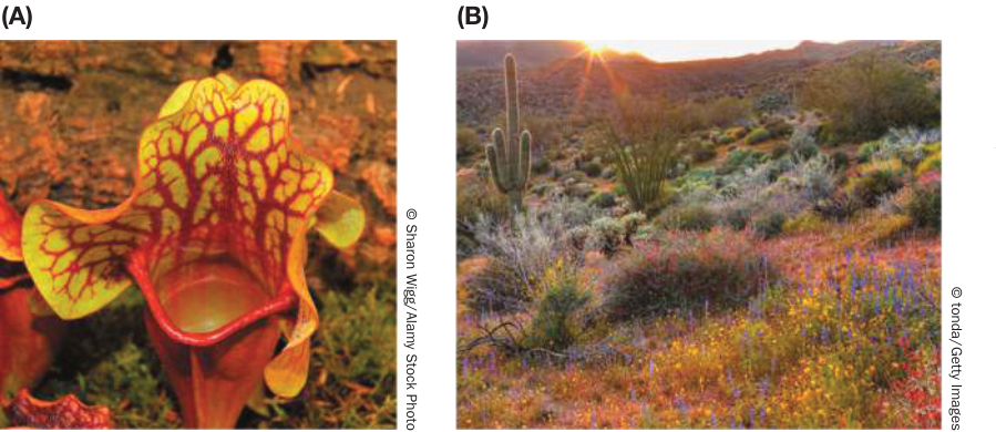
Figure 55.1 Defining Communities Communities exist at a variety of spatial scales. The community within a single pitcher plant (Sarracenia Purpurea) contains microorganisms and tiny invertebrates (A), whereas a desert community might contain plants and animals over a large, hard-to-delineate, geographic area (B).
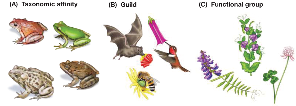
Figure 55.2 Subsets of Species in Communities Ecologists often use subsets of species to define communities. (A) All the amphibian species in a community could be grouped together by taxonomic affinity. (B) All the species that use pollen as a resource form a guild. (C) All the legumes (e.g., vetch, clover, and peas) that have nitrogen-fixing bacteria could be placed in the same functional group. Species within functional groups may or may not use the same resources. (A) Taxonomic affinity
Food web depictions can sometimes include nontrophic interactions such as competition and positive interactions (mutualisms and commensalisms). These so-called interaction webs provide a more realistic view of all the species interactions that might be important in the community. Overall, the food web concept, regardless of whether it includes nontrophic interactions, is a useful visual representation of the important consumer relationships in a community. You will learn more about food webs later in this chapter and in Chapter 56.
Species diversity and composition are important descriptors of community structure
Communities vary widely in species number and species composition (the kinds of species) present. A coral-reef community in the Great Barrier Reef, for example, has many more species of fish than one in the Caribbean. As you saw in Chapter 52, ecologists have devoted considerable effort to measuring the variation in species diversity and species composition at multiple spatial and temporal scales (see Figure 52.12). Patterns at the community or local scale are important descriptors of what ecologists call community structure. Documenting community structure is an important first step in generating hypotheses about how communities work. Let’s first consider the different ways that one metric of community structure—species diversity—is measured.
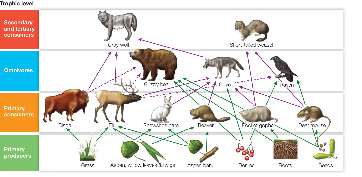
Figure 55.3 Food Webs Show Trophic Interactions in a Community This simplified food web for the meadows and forests of Yellowstone National Park includes only some vertebrates and the plants on which they depend. The arrows show trophic interactions and energetic connections. Herbivores whose sole source of food is plants (green arrows) are primary consumers. Carnivores that kill and eat animals (purple arrows) are secondary and tertiary consumers. Omnivores such as grizzly bears, coyotes, and ravens eat both plant and animal tissues; ravens and grizzlies also eat carrion (dashed purple arrows), so these species are also scavengers. Activity 55.1 The Major Trophic Levels

We have thus far used the term “species diversity” to describe the number of species in a sample, community, or region, but ecologists have a more technical definition. Species diversity is a measure that combines the number of species (species richness) and their relative abundances compared with that of other species (species evenness).
The contribution of both species richness and evenness to species diversity is illustrated in the following example from Mount St. Helens (Figure 55.4). Imagine that we collect samples of 20 individual amphibians in each of two different ponds on Mount St. Helens 3 years after its eruption. Our sample from Pond A contains 17 individuals of one species (Pacific tree frog, Pseudacris regilla) and only 1 individual of each of the other three species (an uneven distribution). Our sample from Pond B, however, contains 5 individuals of each of four amphibian species (an even distribution of individuals). Even though the species richness of the two communities is the same (four species), Pond A is less diverse because the less abundant species are encountered less frequently compared with the single most abundant species.
There are several ways to measure species diversity quantitatively. One common measure is the Shannon index,
where
= the Shannon index value
= the proportion of individuals found in the th species
= the natural logarithm
= the number of species in the community
The lowest possible value of is zero; higher values represent greater species diversity. Table 55.1 calculates the Shannon index for amphibians in the two Mount St. Helens pond communities shown in Figure 55.4. These calculations show that Pond A has the
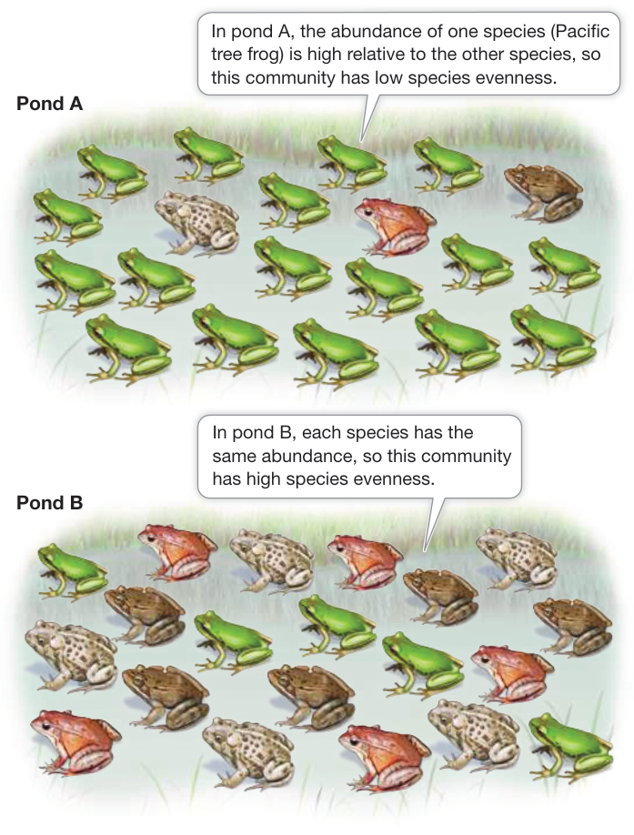
Figure 55.4 Species Richness and Evenness These two hypothetical amphibian pond communities have the same number of species (species richness) but different relative abundance of those species (species evenness). Q: Which pond, A or B, has higher species diversity as measured using the Shannon index (see Table 55.1)? Explain.
Table 55.1 Calculation of Species Diversity for Ponds A and B Using the Shannon Index
| Species | Abundance | Proportion () | ||
|---|---|---|---|---|
| POND A | ||||
| Pacific tree frog | 17 | 0.85 | -0.163 | -0.139 |
| Western toad | 1 | 0.05 | -2.996 | -0.150 |
| Cascades frog | 1 | 0.05 | -2.996 | -0.150 |
| Northern red-legged frog | 1 | 0.05 | -2.996 | -0.150 |
| Total | 20 | 1.00 | -0.589 | |
| POND B | ||||
| Pacific tree frog | 5 | 0.25 | -1.386 | -0.347 |
| Western toad | 5 | 0.25 | -1.386 | -0.347 |
| Cascades frog | 5 | 0.25 | -1.386 | -0.347 |
| Northern red-legged frog | 5 | 0.25 | -1.386 | -0.347 |
| Total | 20 | 1.00 | -1.388 |
To calculate the Shannon index (), the natural logarithm () is applied to for each species ()…
…and then this value is multiplied by once again.
All the values are summed for all the species in the community and multiplied by -1 to get .
Community B has higher species diversity than community A.
lower Shannon index value (), confirming mathematically that this community has lower species diversity than Pond B. Given that both communities have the same species richness, the difference in species diversity is driven by the lower species evenness in Pond A. How does the term “biodiversity” relate to species diversity? Biodiversity is used in reference to various levels of diversity, from genes to species to communities (Figure 55.5). Implicit in this term is the interconnectedness of different scales of diversity. For example, you saw in Chapter 19 that greater genetic diversity can lead to greater fitness of populations, which in turn can promote species diversity. The greater number of different types of communities can also lead to greater diversity at larger regional and continental scales, as you saw in Chapter 52.
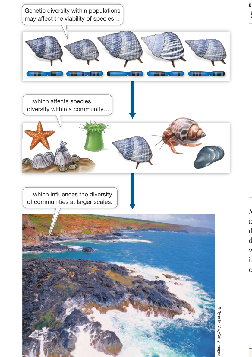
Figure 55.5 Biodiversity Considers Multiple Spatial Scales Diversity can be measured at spatial scales that range from genes to species to communities. The term “biodiversity” encompasses diversity at all of these scales.
Recap and Assess
A community is a group of species that occur together at the same place and time. Communities are often defined by a subset of species based on similar taxonomy, resource use (guild), ecological functions (functional group), or trophic and energetic connections (food webs). Species diversity and composition are descriptors of community structure. Species diversity is a measure that combines the number of species (species richness) and their relative abundances (species evenness). Biodiversity is a term that describes multiple scales of diversity, from genes to species to communities.
- Why are subsets of species used to define communities? What type of community subset was used to define the frogs and toads in ponds on Mount St. Helens?
- What types of species interactions are missing from the food web depicted in Figure 55.3?
- Refer to Table 55.1. Replace the abundance of amphibians in Pond A with the following values (Pacific tree frog = 6, western toad = 8, northern red-legged frog = 4, Cascades frog = 2), recalculate the values in the other three columns in the table accordingly, and then calculate a new Shannon index value. Which pond has the higher species diversity, Pond A or Pond B?
Measuring community structure prompts us to consider many interesting questions about communities. Why do communities differ in the number and composition of species? What processes determine community membership? In the next key concept we will explore how community membership is shaped by which individuals get to the community, deal with the environmental conditions there, and form interactions with other individuals.
Community Membership Depends on Species Supply, Environmental Conditions, and Species Interactions
Learning Objectives
55.2.1 Describe how regional species supply and dispersal ability, environmental factors, and biotic interactions can contribute to community membership.
55.2.2 Explain why studying introduced non-native species provides a unique test of community membership.
Suppose you are looking across the landscape of Mount St. Helens. You see lakes and ponds, alpine meadows, and forests. There is no doubt that these communities vary not only in their species composition but also their species richness. The lakes might be dominated by fishes, amphibians, and freshwater algae; the alpine meadows by various species of grasses, flowering plants, and rodents; and the forests by trees, shrubs, and birds. Even though some species might move from one community to another, the three communities would still be very different. How is it that species come together to form different communities?
Community membership depends on three basic factors: (1) the regional species pool and dispersal ability (species supply), (2)
physical and chemical environmental conditions (abiotic conditions), and (3) species interactions (biotic conditions). Each factor acts as a “filter” that excludes or includes species in particular communities (Figure 55.6). Let’s consider each of these filters in more detail.
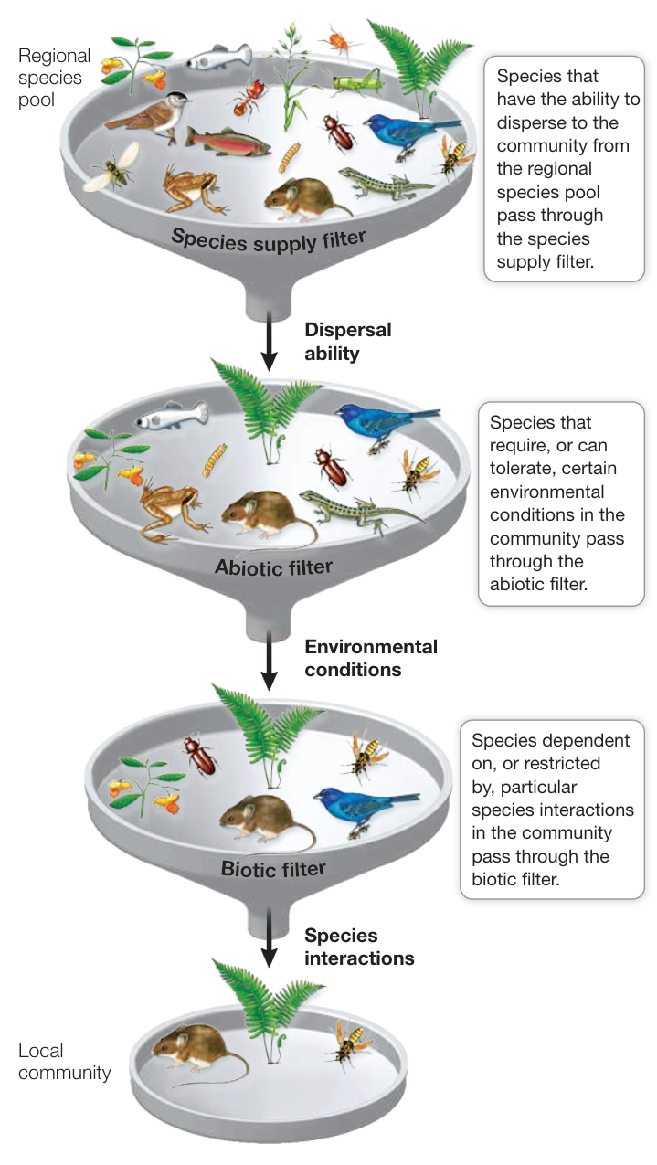
Figure 55.6 Filters Determine Community Membership Species members are included or excluded in a local community by passing through a set of “filters.” Species are lost at each filter, so local communities contain a fraction of the species in the regional pool. In practice, all the filters work at the same time, rather than in series as the figure suggests. (After J. H. Lawton. 2000. Community Ecology in a Changing World. Excellence in Ecology. 11: XI–227. The International Ecology Institute: Oldendorf/Luhe, Germany.) Q: Would it make sense for the fish and frog species in the regional species pool to be present in the local community shown in the figure? Explain.
Community membership depends on species supply
In Chapter 52 we established that regional species pools provide the upper limits on the numbers and types of species that can live within communities (see Figure 52.12). An obvious first step to community membership is the presence of species at the regional level, and their ability to disperse to the community. For example, as communities started to recover from the Mount St. Helens eruption, they began to gain species supplied from the regional species pool of the Pacific Northwest of North America. Because they were able to disperse to the mountain, these species began to colonize the new and unique environments created in the aftermath of the devastation.
Maybe the best examples of how species supply affects community membership are seen in the introduction of novel species to communities. Humans have greatly expanded regional species pools, allowing new and potentially invasive species to enter communities. Chapter 54 described the catastrophic effects of the unintentional release of invasive lionfishes in Atlantic Ocean and Caribbean coral-reef communities. The lionfish invasion demonstrates that “getting there” is a critical first step to community membership. All it took was the release of these predators, and their extraordinary ability to prey on reef fishes, to dramatically change coral-reef communities.
Environmental conditions are critical to community membership
As you might expect, all species in a regional species pool do not end up becoming members of every community in that region. A species may make it to a community but fail to become a member because of unsuitable environmental conditions there. You might think of the influence of the environment as an “abiotic filter” that restricts species that are physiologically incapable of surviving in a given community. The lakes in the Mount St. Helens area, for example, have environmental attributes that accommodate fishes, amphibians, and aquatic insects but not trees.
The physical environment can be a significant barrier to introduced non-native species. Consider, for example, marine organisms that are often introduced into foreign ports via ballast water (seawater that is pumped into and out of ballast tanks to stabilize large cargo-carrying ships). Ballast water picked up outside one port and then dumped in another can potentially release organisms (from bacteria to planktonic larvae to fishes) that can colonize nearshore communities. While most ballast-water organisms do not survive the thermal, salinity, or light regimes of their new environment, a small percentage are not physiologically constrained by such conditions and may gain a foothold, especially if they are introduced multiple times.
Community membership can shift with changing environmental conditions. For example, growing evidence indicates that climate change—in particular, rising temperatures—may improve conditions for some non-native species, increasing their ability to thrive. Jay Stachowicz and his colleagues found that the recruitment and growth of invasive marine invertebrates known as ascidians (sea squirts) in New England were dependent on warm winter and summer water temperatures (Figure 55.7A). Warmer temperatures gave the non-native organisms an earlier start in spring and increased the magnitude of their growth relative to that of native sea squirts. A similar story can be told for the European green crab (Carcinus maenas), whose recruitment to estuarine communities along the Pacific Northwest coast is dependent on warm water temperatures during El Niño conditions (Figure 55.7B).
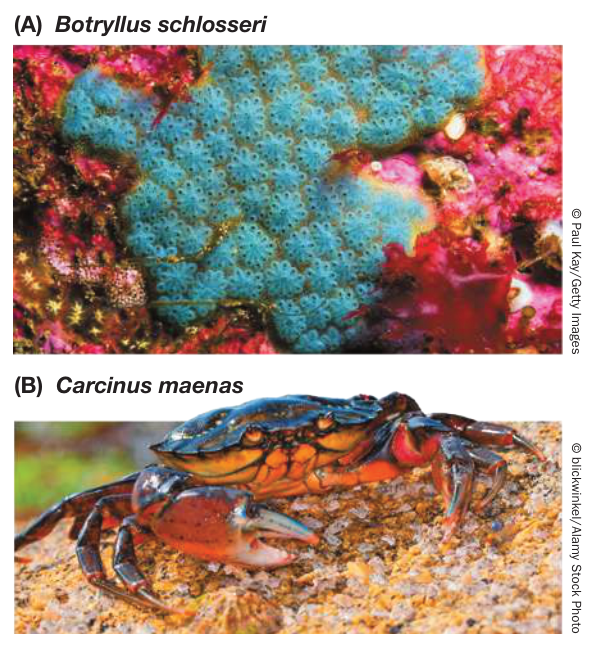
Figure 55.7 Species Invasions Can Depend on Environmental Conditions (A) Invasive sea squirts in New England depend on warmer water temperatures to grow and outcompete native sea squirts. (B) The recruitment of European green crabs to U.S. Pacific Northwest estuaries depends on warm water conditions such as those that occur during El Niño.
The final requirement for species membership is the ability to coexist with other species. Let’s consider the mediating effects of species interactions on the inclusion (or exclusion) of species in communities.
Resident species can restrict or promote community membership
Even if a species makes it to a community and is able to tolerate its environmental conditions, it must be able to live with all the other species in that community. It must be able to obtain food, survive without being eaten, and cope with competitors. Thus whether a species is successful in a new community will depend on the presence of resident species that either promote or restrict species membership.
The ability of resident species to exclude or slow the population growth of non-native species is called biotic resistance. While there are a handful of studies showing that competitors and herbivores can slow down the spread of non-native plant species, confirmed examples of biotic resistance are few. Identifying whether biotic resistance is common in nature may reflect the fact that many failed introductions of non-native species go undetected. Nevertheless, the evidence from the invasive species literature suggests that the influence of resident species may be a fairly porous filter when it comes to restricting species from, or promoting species to, communities.
Recap and Assess
Community membership is a consequence of regional species pools, environmental conditions, and species interactions. These three factors act as “filters” that control community membership. Biotic resistance—the process by which species interactions exclude or slow the population growth of colonizing species—is rarely documented.
- Refer to Figure 55.6. Which factor is most limiting to the species membership of the local community? Explain.
- If you were trying to reduce the number of non-native species colonizing Mount St. Helens, what one best general management action would you employ?
Once a species is part of a community, how is it able to coexist with other species there? In the next key concept we will consider theories and examples that seek to explain how species interactions help form communities of varying composition and diversity.
Communities Are Complex Networks of Species Interactions That Vary in Strength and Direction
Learning Objectives
- 55.3.1 Describe the role of indirect interactions in determining community structure, particularly in the case of trophic cascades.
- 55.3.2 Explain how resource partitioning and disturbance can regulate community structure.
- 55.3.3 Define and compare keystone, foundation, and ecosystem engineering species.
- 55.3.4 Discuss how lottery, or neutral, models explain the role of chance in regulating community structure.
So far we have presented a rather static view of communities as groups of species residing in the same place at the same time. But communities are actually complex networks of species with connections that vary in their strength (i.e., magnitude) and direction (i.e., positive, negative, or neutral). Every species in a community experiences multiple direct and indirect interactions.
Indirect interactions are important to community structure
A direct interaction is one that occurs between just two species. Indirect interactions occur when the direct relationships between two species are mediated by a third (or more) species (Figure 55.8). The addition of a third species to a two-species interaction has the possibility of dramatically changing the outcome of the original interaction.
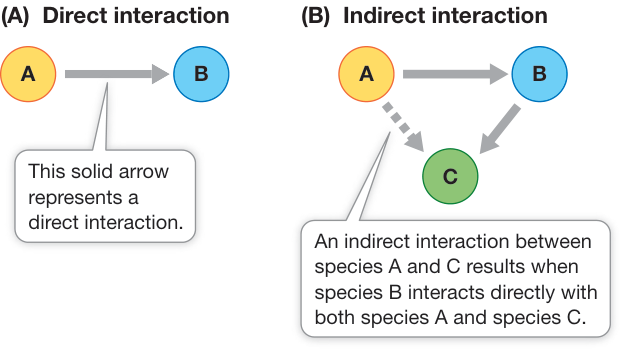
Figure 55.8 Direct and Indirect Species Interactions (A) A direct interaction occurs between two species. (B) An indirect interaction (dashed arrow) occurs when the direct relationship between two species is mediated by a third species.
Indirect interactions were observed by Charles Darwin in On the Origin of Species (1859). Having described the role of bees in flower pollination and seed production of plants in the region of England where he lived, Darwin hypothesized that the number of bees in the region was dependent on the number of field mice that prey on their combs and nests. Noting that mice, in turn, are eaten by cats, Darwin wrote, “Hence it is quite credible that the presence of a feline animal in large numbers in a district might determine, through the intervention first of mice and then of bees, the frequency of certain flowers in that district!”
Today the term “trophic cascade” would be applied to Darwin’s observations. A trophic cascade occurs when the rate of consumption at one trophic level results in a change in species abundance or composition at lower trophic levels. For example, a carnivore eats an herbivore (a direct interaction) and decreases its abundance, causing an indirect positive effect on the primary producer eaten by the herbivore. One example of a trophic cascade is the indirect regulation of U.S. Rocky Mountain meadow and forest communities by wolves, which were reintroduced into Lamar Valley in Yellowstone National Park in 1995. William Ripple and his colleagues at Oregon State University have studied this system extensively.
The simplified food web in Yellowstone National Park depicted in Figure 55.3 shows that gray wolves (Canis lupus) in the park feed on elk (Cervus canadensis), bison (Bison bison), and coyotes (Canis latrans). Although they share some of these prey species with coyotes and grizzly bears (Ursus arctos), wolves exert particularly strong effects on the structure and dynamics of the community. We know this mostly because of how differently the community was structured in their absence, after wolves were hunted to extinction in Yellowstone in 1926. In the absence of wolves, the park service culled elk herds to prevent their populations from exploding. In 1968, in response to public pressure, the selective killing was stopped and the elk population rapidly increased (Figure 55.9A). The elk browsed aspen trees so intensely that the number of young trees recruited (added to the population) declined precipitously; once elk culling stopped, no new trees were recruited at all (Figure 55.9B). The elk also
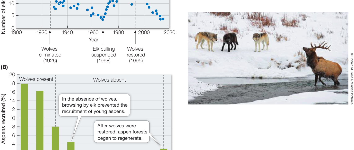
Figure 55.9 Wolves Initiated a Trophic Cascade in Yellowstone National Park (A) Number of elk in Wyoming’s Yellowstone National Park. (B) Aspen recruitment (new trees) in the presence and absence of wolves. (A after W. J. Ripple and R. L. Beschta. 2004. BioScience 54: 755–766; B after J. Halofsky and W. Ripple. 2008. Forestry 81: 195–207.)
Media Clip 55.2 How Wolves Change Rivers Life12e.com/mc55.2
severely browsed streamside willows, with the result that beavers (Castor canadensis), which depend on willows for food, were mostly gone from Lamar Valley. In regions of the park where elk were absent, however, aspen and willow trees flourished. This observation suggested that the decline of the trees in Lamar Valley was indeed due to elk browsing rather than to climate conditions or other factors.
In 1995, after wolves had been absent for 70 years, park managers reintroduced them to Yellowstone, and their population grew rapidly. The wolves preyed primarily on elk. The elk population of Lamar Valley dropped, and elk avoided the aspen groves, where they were especially vulnerable to wolf predation. Young aspen began to grow, willows regrew along streams, and the number of beaver colonies increased from one in 1996 to seven in 2003. Thus the presence or absence of a single predator influenced not only populations of its prey but also, indirectly, its prey’s food resource and other species that depended on that resource. It is clear that wolves have a dramatic effect on the structure of meadow and forest communities through the trophic cascade they create.
Strongly interacting species often regulate community structure
The example of wolves in Yellowstone National Park offers clear evidence that species interactions vary considerably in their strength and direction, influencing the structure of communities. Some species have strong negative or positive effects on community structure, while others may have almost no effect at all. We can measure the interaction strength, or the effect of one species on the abundance of another species, by experimentally removing the “interactor” species and observing the response of the “target” species. If removing the interactor species causes a sharp decline in the population of the target species, we know that the interaction is a strong positive one. Alternatively, the interaction is strongly negative if the removal results in a large increase in the target species. If the removal has little or no effect on the abundance of the target species, then there is no interaction.
Some species can have strong negative effects on a community by excluding or diminishing populations of other species through competition for limiting resources. As we discussed in Key Concept 54.3, competition is often asymmetrical: one species can be more negatively affected by the interaction than another. Asymmetrical competition leads either to competitive exclusion of the more negatively affected species (resulting in fewer species in the community than would be predicted by environmental conditions or dispersal alone) or to various mechanisms that promote coexistence, such as resource partitioning (the sharing of limiting resources by using them in different ways), thus promoting coexistence (see Key Concept 54.3 for the bee-shin dagger agave example).
Competition among species can also be mediated by factors that affect the dominant species’ ability to acquire resources, so-called resource-mediated coexistence. For example, if events in the physical environment such as disturbance or stress affect the growth or survival of a dominant species, competitively inferior species may gain access to limiting resources. We will consider some specific examples of disturbance and stress in Key Concept 55.4. Here we consider how those effects can influence community structure.
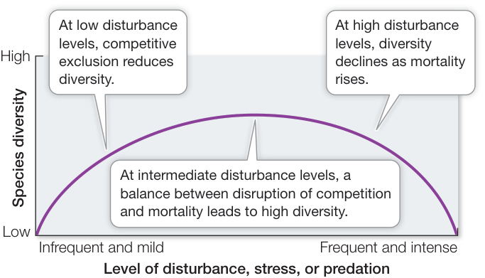
Figure 55.10 The Intermediate Disturbance Hypothesis Species diversity is expected to be greatest at intermediate levels of disturbance (an abiotic process that injures or kills individuals). (After J. H. Connell 1978. Science 4335: 1302–1310.)
The intermediate disturbance hypothesis describes how varying degrees of disturbance (an abiotic process that injures or kills individuals) affect species diversity in communities (Figure 55.10). Joseph Connell, the author of the classic work on barnacle competition (see Key Concept 54.3), noted that the level of disturbance (both frequency and intensity) experienced by a community could have strong effects on its species diversity. He hypothesized that species diversity would be greatest in communities with intermediate disturbance and lowest in communities with low or high disturbance. At low levels of disturbance, competition from dominant species would lead to competitive exclusion of the inferior species, resulting in lower species diversity in the community. At the other extreme, a major disturbance would cause high mortality rates, leading to the extinction of some species in the community and resulting in lower species diversity. At intermediate levels of disturbance, species diversity would be greatest because (1) the influence of the dominant species is reduced by the disturbance, allowing the subordinate species to coexist, and (2) the mortality rates are not as high, so extinction events are less likely to occur.
Here we consider three other types of species that have large effects on community structure.
KEYSTONE SPECIES As described in Key Concept 54.2, keystone species can have strong community-wide effects, not because of their size or abundance but because of the important role they play in communities (Figure 55.11). Keystone species mostly act by creating trophic cascades. For example, top predators such as wolves and sea stars are keystone species because they have a large influence over community species richness, abundance, and composition, even though keystone species may be small in size and their abundance is relatively low.
Sea otters (Enhydra lutris) that inhabit kelp forests on the west coast of North America illustrate how important keystone species can be in regulating community structure. Sea otters feed on sea urchins (Strongylocentrotus spp.), which feed on kelp, establishing a trophic cascade. Without predation by sea otters, sea urchin populations can explode, resulting in voracious consumption of kelp. Stretches of nearshore habitat that become nearly devoid of kelp beds, called “urchin barrens,” can no longer support the diversity of life that is supported when kelp habitat is present.
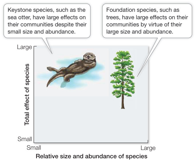
Figure 55.11 Keystone versus Foundation Species Species that have large effects on their communities do so by virtue of their relative size and abundance. (After M. E. Power et al. 1996. BioScience 46: 609–620.)
FOUNDATION SPECIES Some strongly interacting species are capable of providing habitat and food for other species. These foundation species have a large effect on communities as a consequence of their large size or great abundance (see Figure 55.11). Trees are a good example of foundation species. For example, fig trees in tropical forests provide physical habitat for several thousand species of insects, non-avian reptiles, birds, and rodents in their canopy. Fig trees also serve as an important food source for species by producing fruits several times every year, especially at times when few, if any, other trees are fruiting. Dozens of frugivores depend on figs when no other fruits are present. Fig-eating animals include fruit bats, parrots, toucans, pigeons, flycatchers, trogons, orioles, rodents, howler monkeys, and even fishes, which eat figs that fall into nearby streams. All of these animals represent prey for a diverse community of predators.
ECOSYSTEM ENGINEERING SPECIES Some species are specifically known for creating, modifying, or maintaining physical habitat for themselves and other species. These ecosystem engineering species can be either keystone or foundation species. These are species whose primary effect is to engineer the physical environment (rather than providing food), and they do not necessarily have great size or abundance in the community. For example, beavers create new habitats by cutting down (and killing) trees and using them to dam streams and create ponds and wetlands that provide habitat for species that would otherwise be unable to live in the area (Figure 55.12).
Species with similar effects on one another may coexist by chance
We have thus far discussed instances in which communities are composed of a few strongly interacting species and many weakly interacting species. But sometimes species in a community have relatively similar effects on one another. How is species diversity maintained when species vary little in their ability to obtain resources?
Over the last few decades, ecologists have proposed and tested so-called lottery, or neutral, models that emphasize the role of chance in the maintenance of species diversity. Like the name suggests, these models assume that when resources are made available, they are used at random by individuals of different species who happen to be in the “right place at the right time.” As long as all individuals have similar chances of obtaining resources (or “winning the lottery”), and no clear advantage in dispersal ability or population growth, then their presence in the community should be maintained by chance events that free up resources for individuals competing for those resources. If there is a large disparity among species in their ability to obtain resources, the dominant competitor will always have a greater chance of obtaining resources and will eventually monopolize them. So for lottery models to work, the element of equal chance for all individuals to obtain resources is paramount to coexistence.
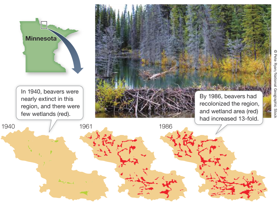
Figure 55.12 Beavers Are Ecosystem Engineers By damming streams, beavers created networks of different types of wetlands (shown in red) in a 45-square-kilometer watershed on Minnesota’s Kabetogama Peninsula, thus increasing species diversity in the region. (Maps after R. J. Naiman et al. 1988. BioScience 38: 753–762.)
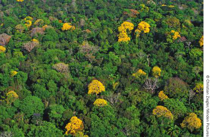
Figure 55.13 Lottery Models Emphasize the Role of Chance Highly diverse tropical rainforests have hundreds of tree species that overlap in their resource requirements. As long as all individuals have similar chances of obtaining those resources (or “winning the lottery”), and no clear advantage in dispersal ability or population growth, then their presence in the community should be maintained by chance events.
The role of chance in maintaining species diversity, especially in unpredictable environments, has intuitive appeal. As long as individuals of species win the lottery every once in a while, they will continue to reproduce and grow their population. Lottery models have most often proven useful when applied to highly diverse communities such as coral-reef fishes and tropical rainforest trees, where hundreds of species overlap in their resource requirements (Figure 55.13).
Ecologists are pursuing various, and sometimes conflicting, hypotheses to explain why certain species coexist in space and time. It is unlikely that any one theory can provide a wholly satisfactory explanation of the mechanisms that drive structure in all communities.
Recap and Assess
Communities are complex networks of direct and indirect species interactions that vary in strength and direction. Trophic cascades, resource partitioning, and intermediate disturbance have been proposed to explain species diversity through their mediation of strong species interactions. Some of those strongly interacting species include keystone species, foundation species, and ecosystem engineering species, which regulate community structure through their interactions with other species. In communities where species interactions are more equivalent, chance plays a greater role in determining community structure.
- Suppose wolves were once again excluded from Yellowstone National Park. What direct and indirect interactions would change, and what effect would this have on aspen forests?
- Make an argument for why beavers could be considered ecosystem engineering species and keystone species but not foundation species.
- Using the lottery model as your guide, explain how species that depend on the same set of limiting resources can coexist.
When Mount St. Helens erupted in 1980, it was clear that the surrounding ecological communities would change forever. Change is a regular feature of all communities, but not all changes are as dramatic as those involving a volcanic eruption. In the next key concept we will consider how both subtle and catastrophic factors change communities over time.
Communities Are Always Changing
Learning Objectives
- 55.4.1 Explain how disturbance, stress, and abiotic factors contribute to community change.
- 55.4.2 Describe the difference between primary and secondary succession in communities.
- 55.4.3 Explain how facilitation and inhibition influence succession in communities.
- 55.4.4 Discuss the concept of alternative states, or regime shifts, including how such states might arise.
Imagine that you could look back in time and observe the change in a typical forest on Mount St. Helens (Figure 55.14). Over the last few decades, you would have seen both subtle and catastrophic changes. Subtle changes would involve a slow replacement in species composition as a consequence of competition, predation, and facilitation. More catastrophic changes would include volcanic eruptions and deforestation, resulting in the destruction of some species and replacement with others over time. The community at any one time is the result of these various changes both natural and human-caused.
Change in communities can be caused by abiotic and biotic factors
How a community changes in species composition over time is known as succession. Succession is the result of both abiotic (physical and chemical) and biotic factors.
A disturbance is an abiotic event that physically or chemically injures or even kills some individuals, creating opportunities for other individuals to grow and/or reproduce. Some ecologists also consider biotic events, such as elephants trampling vegetation or beavers felling trees, to be disturbances. The magnitude of a disturbance can vary enormously. Many disturbances are limited to small areas—for example, a log carried by waves may crush algae and animals on a rocky shore. In contrast, hurricanes, forest fires, and volcanic eruptions can affect communities over hundreds or thousands of hectares. Although small-scale disturbances are far more frequent, the occasional large-scale event is often responsible for most of the changes in a community. For example, a single volcanic eruption on Mount St. Helens felled many more trees than multiple storm events ever did, even over decades.
Stress, in contrast to disturbance, occurs when some abiotic factor reduces the growth, reproduction, and/or survival of some individuals. A common stress on the mountain communities of Mount St. Helens is the effect of temperature on the growth and reproduction of plants. As temperatures decrease with increasing elevation on the mountain, you might expect plants at higher elevations to experience more stress than those at lower elevations. But as illustrated in Figure 54.14, the stress that alpine plants experience at higher elevations can be tempered by the presence of neighboring plants. That is, some types of interactions can mitigate the effects of stress.
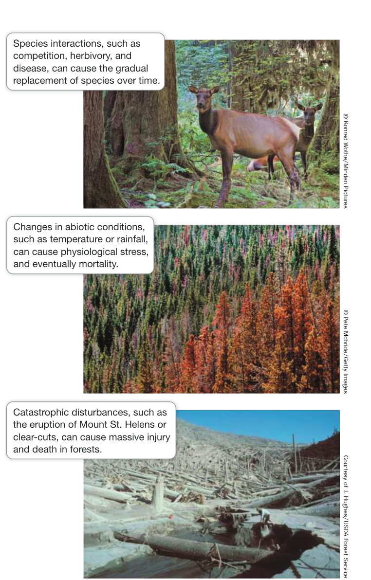
Figure 55.14 Changes on Mount St. Helens Forest communities on Mount St. Helens have experienced significant changes over hundreds of years. The types of change have been both subtle and catastrophic.
Biotic factors can influence community change as well. On Mount St. Helens, change might be driven by competition among different tree species, with the most dominant tree species surviving over time (see Figure 55.14). Herbivory by elk is another example of a species interaction that can initiate change. By preferentially browsing on certain species such as willow and aspen, elk can shift the trajectory of plant community succession from forest to meadow, as happened in Yellowstone National Park (see Figure 55.9).
Succession is a process of change in communities over time
Traditionally ecologists have viewed succession as a progression of stages in which species come and go until a climax community arises. The climax community is thought to be a stable assemblage of species that experiences little change until an intense disturbance wipes out the community, sending it back to its initial stages again. As you will see later in this key concept, whether some communities reach a true stable end point is questionable. Let’s consider the mechanics of succession in more detail.
Succession is probably most easily observed after a catastrophic disturbance kills all the organisms in a community, leaving an environment devoid or nearly devoid of life. This type of change is known as primary succession. Glaciers, volcanic activity, and in some cases floods or landslides cause disturbance that initiates primary succession. Primary succession by its very nature can be slow because the early arrivals (known as pioneer or early successional species) must deal with extreme conditions. Many pioneer species deal with these conditions by employing certain life history strategies or species interactions to their favor.
Connect the Concepts Key Concept 53.3 describes how life history strategies are the lifetime patterns of growth, reproduction, and survival of a species. Pioneer species tend to have life history strategies that maximize population growth (r-strategists).
One of the best-known examples of primary succession is that seen in plant communities in the wake of the retreat of glaciers in Glacier Bay, Alaska (Figure 55.15A). Captain George Vancouver first recorded the location of glacial ice there in 1794, while exploring the west coast of North America. Over the last 200 years, the glaciers have retreated up the bay, scraping the landscape down to bare rock and leaving a series of moraines—gravel deposits dropped where the glacial front was stationary for a number of years. No human observer was present to observe changes over the entire 200-year period, but ecologists have inferred the temporal pattern of succession by studying the vegetation on moraines of different ages (Figure 55.15B). The youngest moraines, closest to the current glacial front, are populated with bacteria, fungi, and photosynthetic microorganisms that can support themselves on bare rock. Slightly older moraines farther from the glacial front are home to pioneer communities containing lichens, mosses, willows, and cottonwoods, which break down rocks and, when they die, decompose and contribute to the buildup of soil. Mosses and a few species of shallow-rooted shrubs in the genus Dryas eventually become established and contribute to soil building as they die and decompose. Still farther from the glacial front, successively older moraines have deeper soil layers that support shrubby willows and alder trees. Finally, a century after glacial retreat, a mature Sitka spruce (Picea sitchensis) forest dominates, fostering a diverse array of forest species.
Nitrogen is virtually absent from glacial moraines, so the plants that grow best on recently formed moraines at Glacier Bay are Dryas and alders, both of which have nitrogen-fixing bacteria in nodules on their roots (see Figure 34.8B). Nitrogen fixation by these plants improves the soil so that spruce trees can grow (see
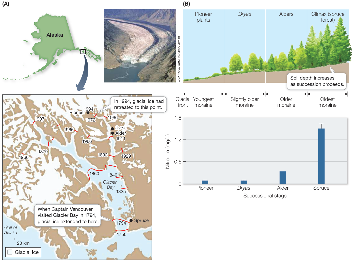
Figure 55.15 Succession in Glacier Bay, Alaska (A) Over more than 200 years, the melting of glaciers has exposed bare rock and glacial moraines to colonization and succession. (B) As the community occupying a glacial moraine changes from an assemblage of pioneer plants such as Dryas to a spruce forest, soil depth increases and nitrogen accumulates in the soil. (After F. S. Chapin et al. 1994. Ecol Monograph 64: 149–175.) Q: Based on the locations of the glaciers over time, describe where the oldest and youngest communities (black dots) are located.
Figure 55.15B). Spruces then outcompete and displace the early colonists. If the local climate does not change dramatically, a climax community dominated by spruce trees is likely to persist for many centuries on old moraines at Glacier Bay.
On Mount St. Helens, ecologists have had a unique opportunity to study primary succession from its inception. As described in the opening story, the alpine communities surrounding the lava dome experienced the greatest destruction; they were the first to be hit by an avalanche of mud and hot water and then pelted by hot, sterilizing pumice. This created the so-called Pumice Plain, an area completely lacking life, including any traces of organic matter. The first plant species to arrive, a year after the eruption, was the dwarf lupine (Lupinus lepidus). Dwarf lupines, like Dryas and alders, use the nitrogen produced by bacterial symbionts in root nodules to colonize the sterile environment of the Pumice Plain. They subsequently facilitated other species of plants by trapping seeds and detritus and increasing the overall nutrient content of the soil. By providing safe sites for seedlings to become established, the dwarf lupines greatly increased the rate of primary succession on Mount St. Helens. Because of the early inroads made by dwarf lupine, researchers documented roughly 20 plant species living on the Pumice Plain 20 years after the eruption.
A surprising discovery about primary succession on Mount St. Helens was the important role of animals in directing change. For example, scientists observed that newly formed and isolated ponds and lakes were colonized by amphibians at a faster rate than one might predict given the surrounding harsh conditions. Ecologists discovered that frogs and salamanders were using tunnels created by the northern pocket gopher (Thomomys talpoides) as refuges when they made their way from pond to pond across the dry landscape (Figure 55.16). Pocket gophers successfully survived the eruption by living in tunnels under the mud. They also benefitted by the expansion of their preferred habitat—grassy meadows—after the eruption. Pocket gophers facilitated plant succession through their burrowing activities, which brought to the surface organic matter, seeds, and fungal spores buried deep under the pumice.
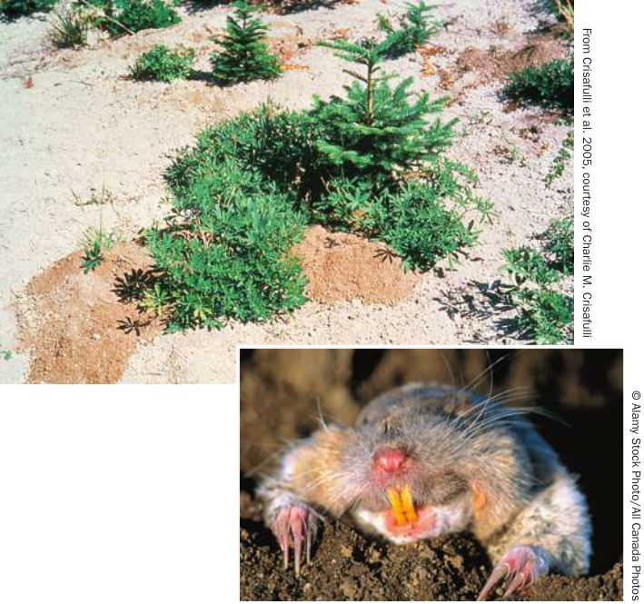
Figure 55.16 Pocket Gophers to the Rescue The burrowing activity of northern pocket gophers, some of which survived the eruption underground, resulted in tunnels that amphibians used to move from one pond to another. It also brought organic matter, seeds, and fungal spores to the soil surface, creating microhabitats, like this one in the Pumice Plain, where plants can grow. Q: Are pocket gophers keystone species, foundation species, or ecosystem engineering species?
The other type of succession, known as secondary succession, involves the reestablishment of a community when most, but not all, organisms have been destroyed. Secondary succession is often initiated by human activities (such as clear-cutting) as well as by natural disasters (such as storms and fires). Secondary succession is more common, and it progresses more rapidly than primary succession. For example, even though the eruption of Mount St. Helens completely destroyed some areas near the blast zone, there were large areas where organisms survived and secondary succession took place.
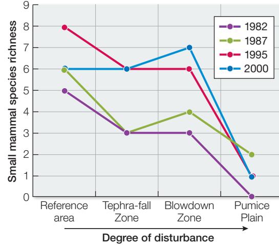
Ecologists compared primary and secondary succession on Mount St. Helens by following small mammals in the community. As we mentioned in the chapter opening, different Mount St. Helens communities experienced different levels of disturbance from the eruption. Investigating Life: Rising from the Ashes describes research by Charles Crisafulli and colleagues at the USDA Forest Service, showing that the recovery of small mammal populations on Mount St. Helens varied significantly between primary and secondary successional habitats. The Pumice Plain (primary successional habitat completely devoid of life after the eruption) had the lowest species richness of small mammals, a pattern that persisted for at least 20 years. In contrast, small mammal populations recovered relatively quickly in the Blowdown Zone and the
Tephra-fall Zone (secondary successional forest in which some life survived under downed trees and ash fall). In fact, within a few years, the number of small mammals in these two zones was similar to that in the undisturbed reference area 21 kilometers away. This comparison makes clear that the starting conditions characterizing secondary succession are critical in giving communities a “head start” in their recovery.
Both facilitation and inhibition influence succession
The progress of succession greatly depends on the activity of successive colonists, each of which modifies the environment to either facilitate or inhibit the colonization by other species. Facilitation is seen, for example, in the fixation of nitrogen by Dryas and alders that allows spruce trees to become established in Glacier Bay (see Figure 55.15B). At later stages of succession, though, competition by spruce trees for nitrogen, light, and water inhibits other tree species from establishing themselves. Likewise, dwarf lupines helped facilitate the establishment of later successional plants but, in turn, were inhibited by multiple insect herbivores, which were able to control the pace of primary succession.
Why do we see this interplay between facilitation and inhibition as succession progresses? In most post-disturbance successional sequences, the early pioneer species are exposed to physically challenging conditions that can be tolerated only with the help of other species. For example, in secondary succession, many of the first organisms to arrive on bare soil after a disturbance are detritivores, which process dead organic matter and release nutrients, thus facilitating the establishment of early colonizing plants. Early successional species that can disperse to these habitats and tolerate and modify the abiotic environment will likely facilitate other species without those capabilities. As succession progresses, species that are less stress-tolerant but are larger, longer-lived, and competitively superior will likely come to dominate as the conditions improve, inhibiting earlier pioneer species. While there is typically a transition from early facilitation to later inhibition in most successional sequences, as species diversity increases, a variety of both positive and negative interactions naturally arise, further shaping the pattern of succession.
Alternative successional pathways result in variations in community composition
The trajectory of succession in any community is not necessarily a repeatable and predictable process. Succession often occurs over long periods of time—longer than the life span of any one researcher—making it hard to know whether the changes in species composition are repeatable over time. For example, suppose dwarf lupines had not successfully colonized the Pumice Plain of Mount St. Helens because of intense herbivory. Might later successional stages, such as growth of Douglas fir forests, never develop? Possibly. What is the chance that different, alternative communities could be established after a similar disturbance? Ecologists use the term alternative states to refer to the different community assemblages that could develop at the same location under similar environmental conditions.
The theory behind alternative states can be visualized by imagining a landscape full of valleys, each of which represents a
Investigating Life: Rising from the Ashes
different community type or state (Figure 55.17A). Imagine, for example, valleys on the Pumice Plain of Mount St. Helens, each of which represents a community that might potentially form there. Impose upon this landscape changes in local conditions—such as the presence or absence of a particularly strongly interacting species—that might influence a community to migrate out of one valley (or state) and into another (Figure 55.17B). Intense grazing by herbivores could, for example, influence where dwarf lupine becomes established on the Pumice Plain. If lupine does not become established in a “new” valley, a different successional trajectory may be established, leading to an alternative state for the community. Now, what if conditions change again, and revert back to those of the initial state? Interestingly, even if original conditions are restored, the community may not revert to the initial state. If the change experienced by the original community was sufficiently large, the successional trajectory of the community can be irrevocably changed (Figure 55.17C). For example, removing herbivores from the system might not bring back dwarf lupine. The system is said to show hysteresis when the community is unable to shift back to its initial state even when the original conditions are restored.
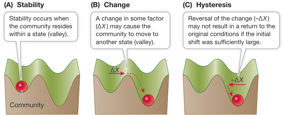
Figure 55.17 Alternative States (A) A community is represented by a ball that moves within a landscape of community states (valleys). (B) In this analogy the valleys are shallower or deeper according to the magnitude of change ( ) needed to shift the community from one state to another. (C) Hysteresis occurs when reversal of the change ( ) does not return the community to its original state. (After B. E. Beisner et al. 2003. Front Ecol Environ 1: 376–382.)
Experiment
Original Paper: C. M. Crisafulli et al. 2005. Small mammal survival and colonization on the Mount St. Helens Volcano: 1980–2002. In Ecological Responses to the Eruption of Mount St. Helens. V. H. Dale et al. (eds.), pp. 199–218. Springer: New York.
Charles Crisafulli and his colleagues were some of the first ecologists to study the successional processes on Mount St. Helens after the eruption. They concentrated on the recovery of small mammals in three types of communities that the eruption had disturbed in different ways: a primary successional community named the Pumice Plain, which experienced complete destruction of all living things, and two secondary successional communities: the Blowdown Zone, in which trees fell and the area was covered in mud but some life remained underground, and the Tephra-fall Zone, where the intact forests and meadows were covered in volcanic debris.
An undisturbed reference area, 21 kilometers away from the mountain, was used as a control. To compare the initial survival and subsequent recovery of small mammals in primary versus secondary successional communities, the researchers conducted extensive trapping between 1982 and 2000 at several locations on
Mount St. Helens and in the reference area.
HYPOTHESIS As a result of the variation in disturbance from the eruption, the primary successional community will have lower mammal species richness than the secondary successional communities, or the reference area, both initially and through time.
METHOD
- Starting in 1982, several sites were established in the reference area and in three volcanically disturbed areas (Pumice Plain, Blowdown Zone, and Tephra-fall Zone). Trapping sessions were conducted at the sites up to four times a year, from June to October.
- At each site, live traps baited with rolled oats and peanut butter were set up in multiple plots in a grid pattern. To capture northern pocket gophers, which remain underground, PVC pipe traps were constructed and placed in their burrows.
- During a trapping session, the traps were checked each morning. Captured animals were identified, uniquely marked, weighed, examined to determine sex and reproductive conditions, and released.
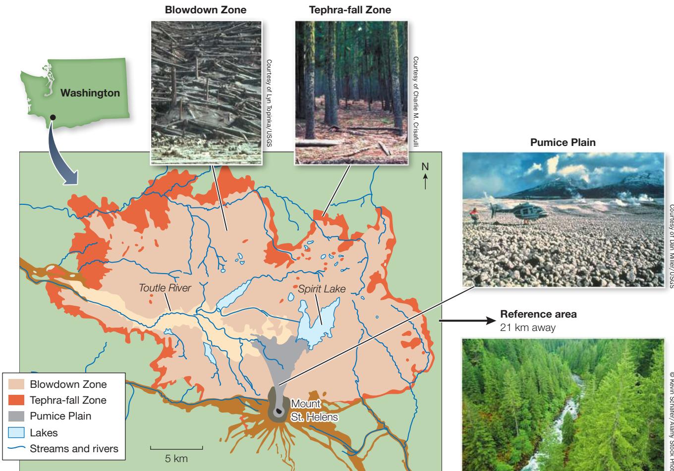
RESULTS Early trapping efforts showed that a total of 17 species of small mammals survived the eruption, with most located in the reference area. Over time, small mammal species richness increased in all the communities but proportionally more so in the Blowdown and Tephra-fall Zones (see graph). By 2000, the two secondary successional communities had species richness values roughly equivalent to those in the reference area. The Pumice Plain had only one year (1987) when more than one species of small mammal was present.
CONCLUSION Numerous small mammal species survived and thrived in the post-eruption secondary successional communities of Mount St. Helens. In comparison, the primary successional community showed little recovery of small mammal richness over the 20-year period.
Work with the Data
In addition to examining small mammal species richness, Crisafulli and his team were interested in the composition of those species and their abundance—data that could give them additional insights into the processes important to the species’ recovery (or lack thereof). The table shows capture data from 2000 on the small mammal species composition and proportional abundance in the four different post-eruption communities.
| Small mammal species | Proportion of Individuals | |||
|---|---|---|---|---|
| Pumice Plain | Blowdown Zone | Tephra-fall Zone | Reference area | |
| Deer mouse ( Peromyscus maniculatus ) | 1.00 | 0.20 | 0.25 | 0.10 |
| Yellow-pine chipmunk ( Tamias amoenus ) | 0 | 0.40 | 0 | 0 |
| Cascade golden-mantled ground squirrel ( Spermophilus saturatus ) | 0 | 0.05 | 0 | 0 |
| Creeping vole ( Microtus oregoni ) | 0 | 0.10 | 0 | 0 |
| Shrew mole ( Neurotrichus gibbsii ) | 0 | 0.05 | 0 | 0 |
| Trowbridge’s mole ( Sorex trowbridgii ) | 0 | 0.10 | 0 | 0.05 |
| Montane shrew ( Sorex monticolus ) | 0 | 0.10 | 0.15 | 0.10 |
| Southern red-backed vole ( Clethrionomys gapperi ) | 0 | 0 | 0.45 | 0.65 |
| Townsend’s chipmunk ( Tamias townsendii ) | 0 | 0 | 0.05 | 0 |
| Ermine ( Mustela erminea ) | 0 | 0 | 0.05 | 0 |
| Northern flying squirrel ( Glaucomys sabrinus ) | 0 | 0 | 0.05 | 0 |
| Vagrant shrew ( Sorex vagrans ) | 0 | 0 | 0 | 0.05 |
| Northern water shrew ( Sorex palustris ) | 0 | 0 | 0 | 0.05 |
QUESTIONS►
- Using the data in the table, calculate the species diversity of each of the post-eruption communities using the Shannon index (see Table 55.1). Which community has the lowest species diversity and which has the highest? How does this pattern compare with that of the species richness values for the four communities?
- Plot species diversity versus the degree of disturbance from the eruption for the four communities. How well do the data fit the intermediate disturbance hypothesis (see Figure 55.10)? Explain.
- Consider the presence or absence of particular species in the four communities. Which species is present in all the communities? What does that suggest about its life history?
- The Blowdown Zone, Tephra-fall Zone, and reference area all have similar species richness (7, 6, and 6 species, respectively), but how do they compare in terms of species composition? Do they appear to be similar? If not, why do you think this is the case?
Communities that have undergone alternative states, or what are sometimes called regime shifts, have become increasingly of interest as it becomes clear that human activities, such as habitat destruction, species introductions, and overharvesting, are shifting communities to alternative states. Once communities have shifted to a new regime, it is often unclear whether the original community can be restored or whether hysteresis will occur. Reintroducing wolves to Yellowstone National Park did successfully result in the recolonization of aspen as a consequence of elk population control (see Figure 55.9). But will protection of sea otter populations help reestablish kelp forests? Will Atlantic Ocean and Caribbean coral-reef fish communities recover if lionfishes are eradicated there (see Chapter 54, Investigating Life: The Lionfish King)? These are questions whose answers may be found in better understanding the factors that drive alternative states and the role that restoration plays in reversing the effects of those factors.
Recap and Assess
Communities constantly undergo change in species composition over time as a result of abiotic and biotic factors, a process known as succession. Abiotic-induced changes to communities come in two forms: disturbance and stress. There are two types of succession: primary succession is the recovery of a community after a catastrophic disturbance kills all the organisms in it, and secondary succession is the reestablishment of a community when most, but not all, organisms have been destroyed. Both facilitation and inhibition influence succession. Communities under similar environmental conditions are sometimes subject to alternative successional pathways, leading to variations in community composition (alternative states).
- Describe the types of biotic and abiotic changes that have affected forest communities on Mount St. Helens.
- True or false? “Primary succession is controlled only by facilitation.” Explain your answer.
- Define and give an example from the chapter of an alternative state, or regime shift.
We have focused thus far on the dynamic nature of community structure and on the factors on which community membership depends. In the next key concept we will consider whether the successful functioning of communities depends on the number of species they contain. In other words, how does species richness affect community productivity and stability?
Relationships between Species Diversity and Community Function Are Often Positive
Learning Objectives
- 55.5.1 Summarize the relationship among species diversity, community function, and stability.
- 55.5.2 Describe how and why growing polycultures can increase agricultural productivity.
As more and more species have either become extinct or are threatened with extinction, ecologists are increasingly interested in understanding what a loss in species diversity means for communities and the way in which they function. Let’s next consider research designed to understand how species diversity affects communities as well as agricultural crops.
Community function describes the way a community works and can be measured using metrics such as plant productivity, soil fertility, or water availability. Another measure of how well a community functions is its resistance to (or recovery from) disturbance, known as its stability. Ecologists have hypothesized that communities with more species function better than communities with fewer species. The argument is that no two species in a community uses resources in exactly the same way such that a community with more species will show more complete and efficient resource use. Also, should environmental conditions change, a species-rich community is more likely to contain some species that can persist under the new conditions. Thus a species-rich community should be more stable—that is, less likely to change over time in either productivity or species composition—than a species-poor community. Let’s examine these assumptions with some experiments.
Relationships between Species Diversity and Community Function Are Often Positive
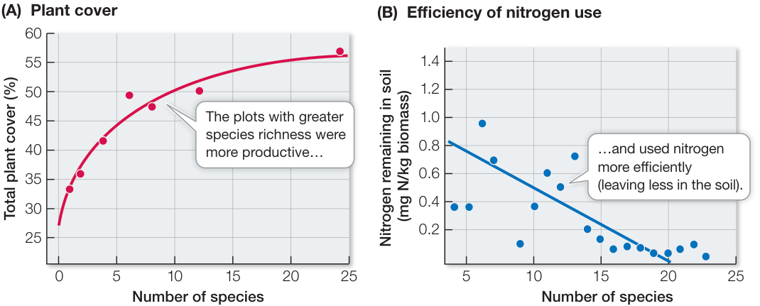
Figure 55.18 Species Richness Enhances Community Productivity David Tilman and his colleagues cultivated a total of 120 grassland plots, containing from 1 to 24 grassland species, for 11 years. (A) Total plant cover (a measure of grass biomass, and thus of net primary production). (B) The amount of nitrogen remaining in the soil is a measure of resource use efficiency. (After D. Tilman, et al. 1996. Nature 379: 718–720.) (B) Efficiency of nitrogen use
Species diversity is associated with productivity and stability
To test the hypothesis that species-rich communities are more stable than species-poor communities, David Tilman and his colleagues at the University of Minnesota cleared 120 outdoor plots, in which they planted grasses in mixtures ranging from 1 to 24 grass species. At the end of each growing season, they measured total plant cover (a measure of grass biomass, and thus of net primary production) and the population densities of all the grasses in each plot. Over a period of 11 years, which included a serious drought, the plots with more species were more productive (Figure 55.18A), and their productivity was less variable from year to year. These findings were consistent with the hypothesis that species richness promotes productivity and keeps productivity stable. Moreover, in the plots with greater species richness, soil nitrogen was used more efficiently (Figure 55.18B). However, the population densities of individual species in the plots were not stable over the years (regardless of a plot’s species richness) because different species performed better during drought years and wet years. In other words, higher species richness increased the stability of plant production in the plots, but not the stability of their species composition.
Researchers continue to debate whether species diversity is responsible for maintaining stability or is simply correlated with stability. This question is important because many of the alterations that humans have made in the structure of natural communities have reduced their species richness, and many of these human-altered communities—notably agricultural communities—are notoriously unstable.
Diversity, productivity, and stability differ between natural and managed communities
Although ecologists have been debating the relationships among species diversity, productivity, and stability for only a few decades, humans have been experimenting with those relationships, albeit inadvertently, for millennia—since plants were domesticated and agriculture was invented. Since the dawn of agriculture, crops have been susceptible to diseases and insect outbreaks: massive (often sudden) increases in populations of species that destroy or damage crops.
The practice of growing crops as monocultures—plantings of a single crop species—is one reason why managed agricultural communities are particularly unstable. Most farmers have little tolerance for the presence of any potential competitors for their crops and actively eliminate weeds (and the herbivore species that live with them) from their fields. Thus a typical agricultural community has very low species diversity. So the answer to the question of whether diversity causes or is merely correlated with stability may be sought in modern farming practices. The predisposition of agricultural communities to play host to outbreaks may well result from human influences on community structure.
For the last 20 years, ecologists have been using traditional subsistence agricultural plots as experimental models for testing the relationships between diversity and stability. Throughout the world, many farmers with small land holdings grow polycultures or multiple crops on the same plot. In Costa Rica, farmers often grow corn together with sweet potato. Such corn—sweet potato dicultures contain fewer sweet potato pests and more parasitoid wasps (which feed on those pests) than do sweet potato monocultures. Wasps feed on the corn pollen, and the tall corn plants act as a structural barrier, shade plant, and source of disruptive chemical signals that interfere with the ability of the sweet potato pests to find their host plants.
Recently, such applications of community ecology have been paying dividends. Although monoculture is overwhelmingly the dominant agricultural practice, polycultures are under development for agricultural production systems as varied as carp and shrimp farming, vermicomposting (raising worms for compost), and biofuel feedstock production.
Recap and Assess
Studies show that the relationships between species diversity and community function (measured as productivity and stability) are often positive. Species diversity enhances productivity because species use resources in slightly different ways; mixtures of species tend to result in a more complete use of limiting resources. Species diversity is hypothesized to enhance stability (a measure of resistance to, or recovery from, disturbance) because the more species a community contains, the more likely some species can persist under variability. These species diversity—community function relationships can be used in agricultural settings to increase crop productivity.
- Why do Costa Rican farmers often grow multiple crops on the same plot, and why might this be a good strategy under drought conditions?
Investigating Life
QA How have ecological communities on Mount St. Helens responded to the eruption, and what processes have been important to their recovery?
A similar question was asked by a group of ecologists who convened a week-long field camp on the twentieth anniversary of the eruption in 2000. Many of the participants had spent their entire careers studying the successional patterns on the disturbed landscapes of the mountain. When they left, they agreed to write a book, and 5 years later Ecological Responses to the 1980 Eruption of Mount St. Helens was published. The book offers unique insights into the successional processes that communities undergo. One important discovery was that the eruption created disturbances that varied in their effects both on the survival of organisms and their subsequent recovery. Because the eruption occurred in spring, many species were dormant under the winter snows and were able to survive the initial eruption. The recovery of some dormant species such as small mammals has been surprisingly quick. A second important discovery was the role that survivors played in controlling the pace and pattern of succession. Unlikely alliances were formed that hastened succession, as you saw with the northern pocket gopher and amphibians. Finally, the researchers realized that multiple mechanisms were responsible for the pattern of succession on Mount St. Helens. Dispersal, abiotic conditions, and species interactions all played a role in the successional process. The variety of ways in which species responded, and the resulting community assemblages, surprised the ecologists lucky enough to have studied the rise of these communities from the ashes.
Future directions
Despite decades of data and discoveries, research on Mount St. Helens has just begun. Will communities there follow paths of succession that are predictable and repeatable? Or will they form alternative states that are highly dependent on their historical legacies? Unfortunately, succession is a long process spanning many lifetimes of scientists. Steps have been taken to continue the “succession” of research on Mount St. Helens. One of the first steps was to secure Mount St. Helens, in 1982, as a National Volcanic Monument dedicated to research, recreation, and education. This designation, along with coordinated research funding, has set the foundation for long-term study sites and data collection and preservation. In addition, the early “pioneer” scientists have cultivated a strong collaborative culture that brings together young scientists who study different levels of biological organization—from molecules to ecosystems. The collaboration is renewed periodically with “science pulse” camps—week-long events attended by dozens of scientists from around the world who gather benchmark data on a diversity of plants, animals, and microbes. Around the campfire at night, the scientists share observations and recruit the next generation of those who will continue the scientific legacy and storytelling into the future.
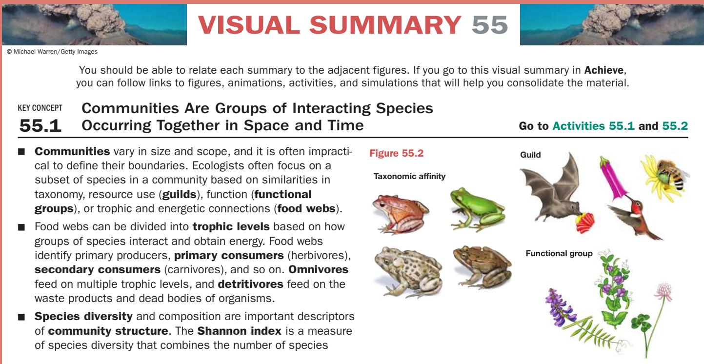
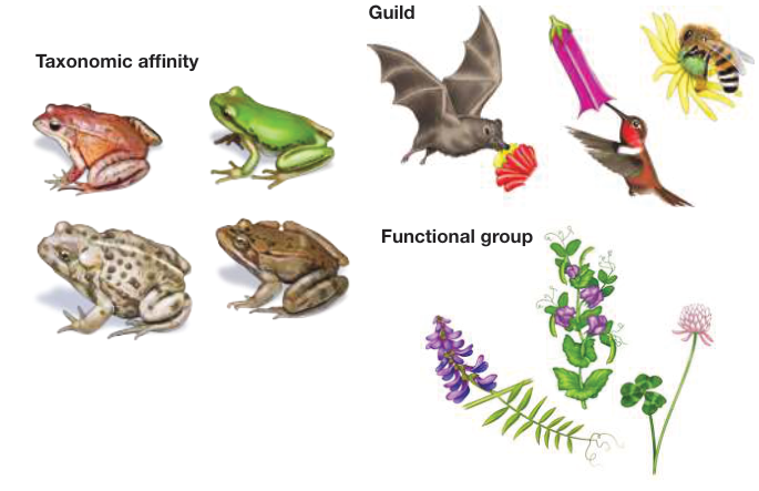
Figure 55.2
Visual Summary
(species richness) and their relative abundances compared with other species (species evenness).
- ■ Biodiversity is a term used to span multiple scales of diversity, from genes to species to communities.
Questions
- What are the different ways ecologists subdivide communities?
- What is a food web, and how does it differ from an interaction web?
- What is species diversity, and how does it differ from biodiversity?
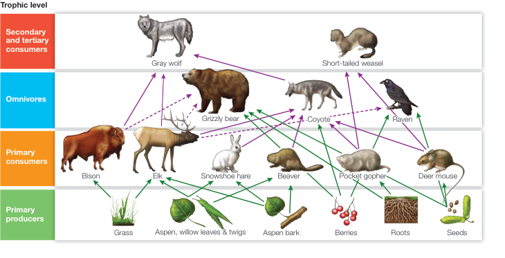
Figure 55.3
Community Membership Depends on Species Supply, Environmental Conditions, and Species Interactions
- ■ The three basic factors responsible for community membership are (1) the regional species pool and dispersal ability (species supply), (2) physical and chemical environmental conditions (abiotic conditions), and (3) species interactions (biotic conditions). These three factors act as “filters” that exclude (or include) species in communities.
Questions
- Which regional scale processes versus local scale processes determine community membership?
- Why is studying introduced non-native species useful in testing community membership?
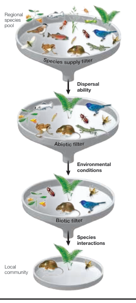
Figure 55.6
Communities Are Complex Networks of Species Interactions That Vary in Strength and Direction
■ Direct interactions occur between two species. Indirect interactions occur when the direct relationships between two species are mediated by a third (or more) species.
■ A trophic cascade occurs when the rate of consumption at one trophic level results in a change in species abundance or composition at lower trophic levels.
■ Some species have especially strong negative effects on community structure, resulting in resource partitioning or resource-mediated coexistence. The intermediate disturbance hypothesis proposes that disturbance promotes species diversity, in part by reducing the negative effects of dominant competitive species.
■ Keystone species influence community structure disproportionally to their size or abundance, producing trophic cascades. Foundation species, by providing food and habitat for other species, have a large effect on communities as a consequence of their large size or great abundance. Ecosystem engineering species affect community structure by creating, modifying, or maintaining physical habitat for themselves and other species irrespective of their size or abundance.
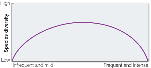
Figure 55.10
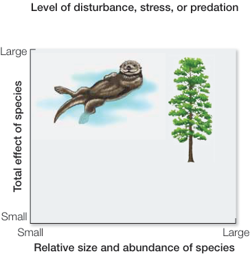
Figure 55.11
- In communities where species interactions are more equivalent, lottery, or neutral, models propose that as long as all individuals have similar chances of obtaining resources, and no clear advantage in dispersal ability or population growth, then their presence in the community should be maintained by chance events that free up resources for competing individuals.
Questions
- How do the indirect interactions of trophic cascades determine community structure?
- How do keystone, foundation, and ecosystem engineering species differ?
- How do resource partitioning, intermediate disturbance, and the lottery model differ?
Communities Are Always Changing
- Communities constantly undergo change in species composition over time as a result of abiotic and biotic factors, a process known as succession. Disturbance and stress are two significant forms of abiotic-induced community change. A disturbance is an abiotic event that physically or chemically injures or kills individuals, whereas stress occurs when some abiotic factor reduces the growth, reproduction, or ultimately survival of individuals.
- There are two types of succession: primary succession is the recovery of a community after a catastrophic disturbance kills all the organisms in it, and secondary succession is the reestablishment of a community when most, but not all, organisms have been destroyed.
- Facilitation and inhibition influence primary and secondary succession.
- The outcome of succession is not always predictable; alternative states, or regime shifts, lead to different community assemblages under similar environmental conditions. Hysteresis occurs when a community is unable to shift back to its original state even when the original conditions are restored.
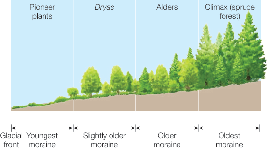
Figure 55.15
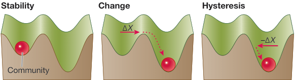
Figure 55.17
Questions
- What are the biotic and abiotic factors that induce change in communities?
- What are the types of succession, and how do they differ?
- Describe alternative states and the process of hysteresis.
Relationships between Species Diversity and Community Function Are Often Positive
- Studies show that the relationships between species diversity and community function (measured as productivity and stability) are often positive. Stability is a measure of resistance to, or recovery from, disturbance.
- Species diversity–community function relationships can be used in agricultural settings to increase crop productivity.
Questions
- How is species diversity associated with community function and stability?
- How can species diversity–community function relationships be used to increase crop productivity?
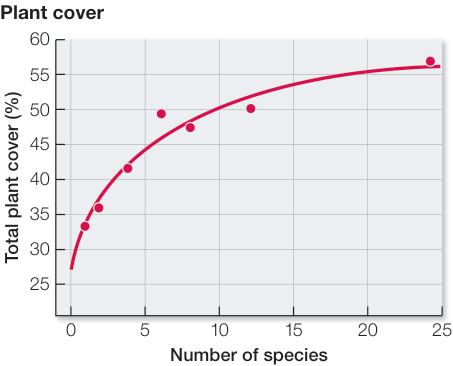
Figure 55.18