Chapter 56Ecosystems
© Cameron Davidson/Gatty Images
Key Concepts
- 56.1 Ecosystem Science Considers How Energy and Nutrients Flow through Biotic and Abiotic Environments
- 56.2 Energy and Nutrients in Ecosystems Are First Captured by Primary Producers
- 56.3 Food Webs Transfer Energy and Nutrients from Primary Producers to Consumers
- 56.4 Nutrient Cycling in Ecosystems Involves Chemical and Biological Transformations
- 56.5 Ecosystems Provide Important Services and Values to Humans
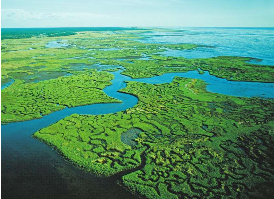
Estuaries, where the river meets the sea, provide food and habitat for commercially important fishes and shellfishes.
Investigating Life: Food Webs in an Acidic and Warming Ocean
There is no dispute that the burning of fossil fuels over the last two centuries has increased Earth’s atmospheric CO2 concentrations. Estimates show that oceans are absorbing about 48% of all atmospheric CO2. Marine primary producers use some of the human-caused CO2 in photosynthesis, but the remainder reacts chemically with seawater, lowering its pH and causing oceans to become more acidic. Ocean acidification can have negative effects on calcifying organisms such as corals, mollusks, and crustaceans, which rely on calcium carbonate for the accretion and maintenance of their external shells. But the negative effects of increasing CO2 and acidification are not universal. For example, primary producers such as phytoplankton, algae, and sea grasses are known to increase their production under elevated CO2. Increasing photosynthesis increases O2 production, which can potentially counteract growing acidity in surrounding seawater. Research is under way on the effects of ocean acidification on single species, but studies on how ocean acidity affects marine ecosystems and food webs are also needed. Moreover, along with the acidification of oceans, water temperatures are rising, potentially creating multiple stressors for organisms.
Estuaries are places where the dual effects of ocean acidification and temperature on primary producers and their food webs may be particularly relevant. Among the most productive ecosystems on Earth, estuaries support a diverse array of marine organisms, including commercially important fish species. Because estuaries are at the interface between land and sea, they have been highly affected by humans through intense overfishing, habitat destruction, and pollution from rivers. Estuaries also experience warm water temperatures, a condition that could intensify with global warming. But estuaries may also be places where the effects of ocean acidification could be mitigated if primary producers such as macroalgae and sea grasses are able to sequester CO2 and provide more food and habitat for higher trophic levels.
Research on estuaries was conducted by a group of researchers on the western coast of Sweden. The group focused on a food web that includes algae primary producers and invertebrate consumers and exposed this food web to different conditions of CO2 and temperature. What they found suggests that ocean acidification and temperature affect food webs in complex ways that may be hard to predict.
Q&A How will food webs respond to the multiple effects of ocean acidification and warming in marine ecosystems? (Find the answer on page 1276.)
Ecosystem Science Considers
Learning Objectives
- 56.1.1 Compare and contrast ecosystems and communities.
- 56.1.2 List sources of energy in ecosystems, and associate each source with the processes that produce it.
- 56.1.3 Explain how nutrients cycle between living organisms and the abiotic environment.
In Chapter 55 we considered communities and the roles that species play in shaping their structure and function. In this chapter we will consider how energy flows and nutrients cycle through communities, a branch of ecology known as ecosystem science. An ecosystem is all the organisms living in a given area and their physical and chemical environment. The term was first coined by A. G. Tansley, a plant ecologist who was interested in how the flow of energy and chemicals was influenced by both the biotic and abiotic components of the environment.
Just like communities, ecosystems occupy a wide range of spatial scales, making them hard to delineate precisely (see Key Concept 55.1). For that reason, ecologists often define an ecosystem using subsets of species and components of the physical and chemical environment based on the questions they are investigating. For example, a soil ecosystem might include only the bacteria that transform nitrogen into forms plants can use. Or an estuarine ecosystem might be confined to the cycling of carbon through a food web of algae and their consumers, as you saw in the opening story.
Energy flowing through ecosystems originates with sunlight and inorganic and organic compounds
The flow of energy through ecosystems comes in a variety of forms (Figure 56.1). The most obvious source is the Sun, which delivers radiant energy that warms Earth and provides energy for photosynthesis. Autotrophs such as plants, algae, and photosynthetic bacteria capture that radiant energy and fix it into organic compounds that make up the tissues of organisms (see Figure 56.1A). Energy can also come from the oxidation of inorganic nutrients by archaea and bacteria through the process of chemosynthesis, which involves using energy from inorganic compounds to take up CO2 and produce carbohydrates (see p. 552). Chemosynthesis typically occurs in ecosystems that lack sunlight and have high concentrations of particular inorganic compounds, such as hydrothermal vents, hot springs, and soils. These two forms of energy capture and carbon fixation are both involved in a process known as primary production. Ecologists use the term “primary productivity” to indicate the rate of primary production over time.
A third source of energy in an ecosystem is the product of primary production—the organic compounds synthesized through photosynthesis and chemosynthesis—that is made available for organisms at higher trophic levels in food webs (see Figure 56.1B). This source of energy, known as secondary production, is contained within the tissues of organisms and is used to power the metabolism of heterotrophs, or the consumers within food webs, which include herbivores, carnivores, omnivores, parasites and pathogens, and eventually decomposers. Metabolism involves converting the organic compounds in food into useable energy—primarily ATP—by processes such as glycolysis (see Key Concept 9.1). The main by-products of metabolism are inorganic compounds, , and water. The energy generated by metabolism to support the “work” that organisms do in their daily life is eventually lost from the ecosystem in the form of metabolic heat.
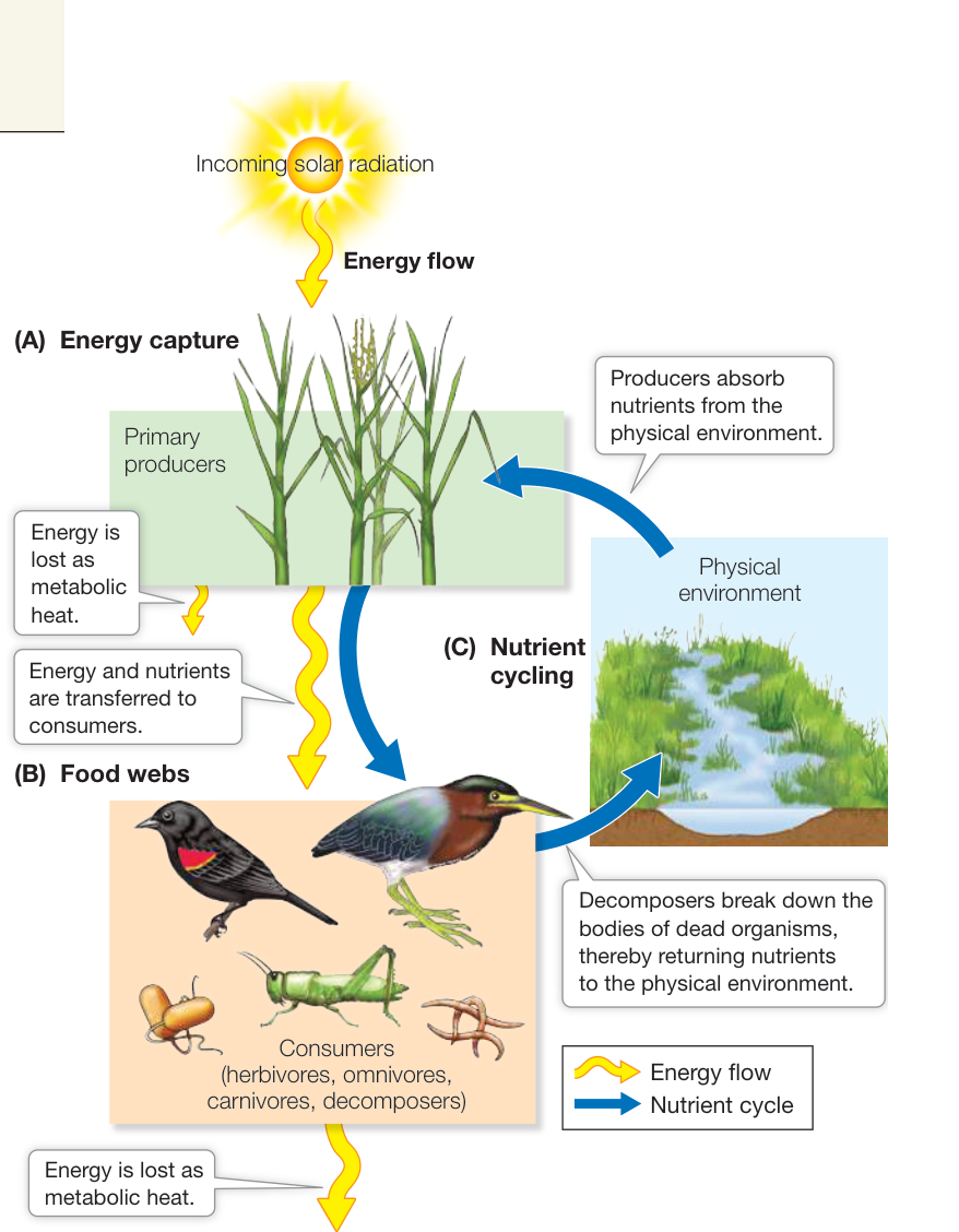
Figure 56.1 Energy Flows and Chemical Nutrients Cycle through Ecosystems (A) The flow of energy through ecosystems comes mostly from the Sun, which delivers radiant energy for photosynthesis by primary producers. (B) Primary producers then provide energy to organisms at higher trophic levels in food webs, but some of that energy is lost as metabolic heat. (C) Nutrients continually cycle between living organisms and the physical components of ecosystems. Q: Why does energy “flow” but nutrients “cycle” through ecosystems?
Nutrients cycling through ecosystems originate in soil, water, and the atmosphere
In contrast to energy, which is ultimately lost from an ecosystem as heat, nutrients continually cycle between living organisms and the abiotic components of ecosystems (see Figure 56.1C). Organisms require 30–40 different nutrients, including the macronutrients carbon, hydrogen, nitrogen, calcium, phosphorus, potassium, and magnesium, and micronutrients such as iron, manganese, zinc, and copper. All the chemical components in the bodies of organisms ultimately originate from soil, water, or the atmosphere, but organisms acquire these materials in many different ways. Autotrophs such as plants take up certain elements directly from soil, water, and the atmosphere and incorporate them in their tissues. Heterotrophs generally acquire elements by consuming the biomass of other organisms, and then reassemble them via chemical reactions. Some heterotrophs acquire some elements from mutualistic microbes that convert them into forms that are usable by their hosts.
Gas exchange by living organisms returns certain elements to the atmosphere as gases. After organisms die, the materials in their bodies become detritus and are broken down by decomposers into simpler biochemical components, which then can be used by autotrophs once again. Elements not used by autotrophs can accumulate in soil, water, or sediments.
Recap and Assess
An ecosystem is all the organisms in a given area and their physical and chemical environment. Autotrophs such as plants, algae, and photosynthetic bacteria capture sunlight and fix it into organic compounds (primary production). Energy is also derived through chemosynthesis: the oxidation of inorganic nutrients by archaea and bacteria. Energy captured through primary production is in turn available for organisms at higher trophic levels in food webs (secondary production). Nutrients continually cycle between living organisms and the abiotic environment.
- An ecologist measures the number of species in an ecosystem. Is she conducting ecosystem science? Explain.
- Describe the two ways that energy and carbon are converted into primary production.
For the remainder of this chapter we will consider in more detail how energy flows and nutrients cycle through ecosystems as depicted in Figure 56.1. We will start with primary production, whereby energy and nutrients are first captured in ecosystems.
Energy and Nutrients in
Learning Objectives
- 56.2.1 Explain the difference between gross primary production and net primary production.
- 56.2.2 Describe the variation in NPP by latitude and biome type in terrestrial and aquatic ecosystems.
- 56.2.3 Explain the factors important to NPP in terrestrial and aquatic ecosystems.
- 56.2.4 Discuss the causes and effects of eutrophication in aquatic ecosystems.
The overwhelming majority of the primary production on Earth comes from photosynthesis. Plants, algae, and bacteria fix carbon by capturing energy from the Sun (or inorganic nutrients, in the case of chemosynthesis) and using that energy to convert carbon dioxide into carbon compounds that can then be used by higher trophic levels.
Net primary production is the amount of carbon remaining in plants after respiration
Fixed carbon, be it from photosynthesis or chemosynthesis, is the currency used to measure primary production. The total amount of carbon fixed by primary producers in an ecosystem is called gross primary production (GPP). Not all GPP becomes living plant matter, or biomass, because primary producers use some of that energy for their own respiration and other metabolic processes. Thus net primary production (NPP), the amount of biomass incorporated into the tissues of primary producers after respiration, is the most common metric used to describe an ecosystem’s carbon fixation. This relationship is represented mathematically as
The carbon not used in respiration is then allocated to such important processes as growth, reproduction, and survival in the face of physical stress, herbivory, or diseases (see Chapter 38).
Patterns of primary production vary with latitude and ecosystem type
Large-scale geographic variation in primary production is one of the most obvious ecological patterns on Earth. Only recently, however, have ecologists been able to reliably quantify patterns of production at global scales. Satellite-based optical sensing techniques now help scientists detect the amount of primary production on land and in the ocean at global scales. How do terrestrial and oceanic ecosystems compare, and how is NPP distributed across the globe?
Estimates of global NPP show that the total amount of carbon taken up by terrestrial ecosystems (52%) is slightly higher than that taken up by the oceans (48%), even though oceans make up a greater percentage (70%) of Earth’s surface. This difference arises because terrestrial ecosystems have a much higher per-area NPP (426 g ) than do oceans (140 g ).
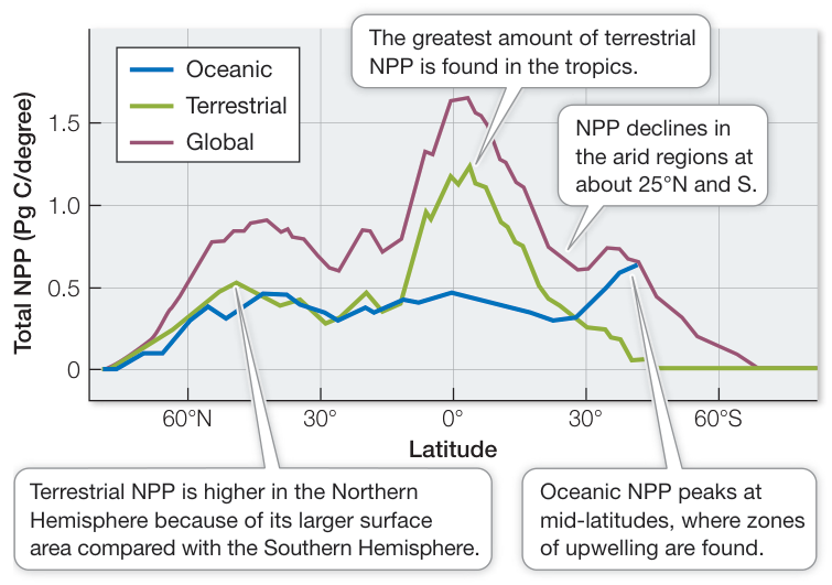
Figure 56.2 Estimates of Total Oceanic, Terrestrial, and Global NPP by Latitude On land, NPP is highest in the tropics and declines at higher latitudes. In the oceans, NPP does not vary much with latitude except at mid-latitudes, especially in the Southern Hemisphere. (1 petagram or g.) (After C. B. Field et al. 1998. Science 281: 237–240.)
Satellite imaging has also shown that NPP is distributed differently on land than in the ocean. NPP on land varies dramatically with latitude, whereas oceans show much less latitudinal variation (Figure 56.2). On land, NPP is highest in the tropics and declines at higher latitudes. Arid regions such as those in deserts ( latitude) and at the poles ( latitude) show extremely low NPP (Figure 56.3A). NPP rises slightly at mid-latitudes, especially in the Northern Hemisphere, where land area is larger than in the Southern Hemisphere (see Figure 56.2). In the oceans, NPP is highest at mid-latitudes and along coastal zones, especially those that experience upwelling (Figure 56.3B). NPP is also higher in the Southern Hemisphere, where ocean area is larger than in the Northern Hemisphere (see Figure 56.2).
Remote sensing has also revealed variation in NPP among different ecosystem types or biomes. Tropical rainforest ecosystems have the second-highest average NPP, even though they make up only a little over 3% of Earth’s surface (Figure 56.4). In comparison, open ocean ecosystems have a low average NPP, despite the large area over which they occur. Some marine ecosystems such as estuaries and algal beds and coral reefs have some of the highest average net primary production, but their small geographic areas make their contributions to global NPP modest. It is important to note, however, that the primary producers in these ecosystems contribute substantially to local and regional NPP and thus are critical to marine food webs.
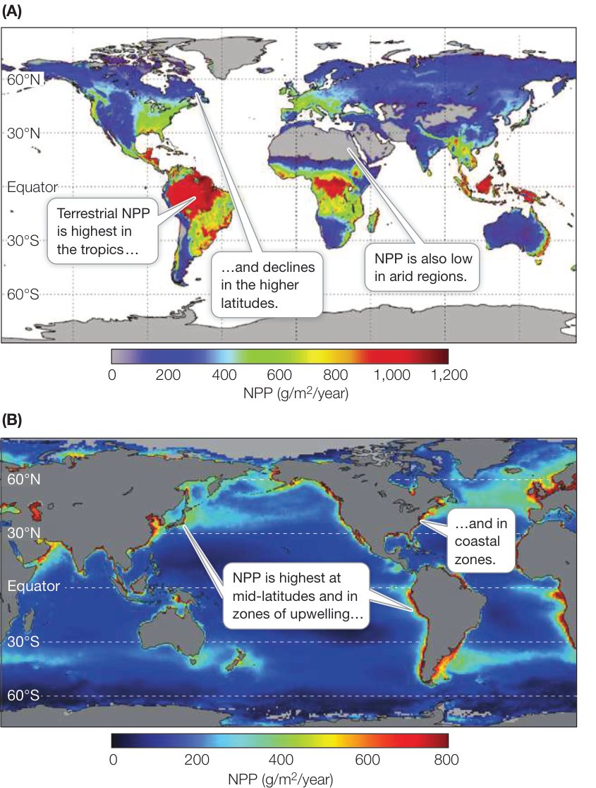
Figure 56.3 Geographic Variation in Terrestrial and Oceanic NPP Maps of NPP based on satellite sensor data. (A) Terrestrial NPP is highest in the tropics and lowest in arid regions and at the poles. Gray areas represent relatively unvegetated land masses, including deserts and ice caps. (B) Oceanic NPP is highest at mid-latitudes and in coastal and upwelling zones. (A, after MODIS GPP/NPP Project [MOD17]. Numerical Terradynamic Simulation Group [NTSG], The University of Montana, Missoula. http://www.ntsg.umt.edu/project/modis/mod17.php; B, image by Robert Simmon, NASA GSFC Earth Observatory, based on data provided by Watson Gregg, NASA GSFC.)
Not surprisingly, the patterns of primary production that we see on land versus ocean, and among ecosystem types, can be explained by separate factors that control primary production in terrestrial versus aquatic systems. We will now consider these factors in more detail—first on land, and then in oceans and lakes.
Precipitation and temperature largely control terrestrial primary production
The strong latitudinal patterns in terrestrial NPP reflect variation in global climate, particularly rainfall and temperature, across latitudes and seasons. NPP increases as average annual rainfall increases up to a maximum (approximately 240 cm per year), but then declines in most ecosystems (Figure 56.5A). The decrease in NPP with high rainfall can occur because of sunlight being reduced by cloud cover over long periods of time or as a consequence of nutrient loss or flooding. NPP also increases with average annual temperature (Figure 56.5B). Thus it makes sense that close to the equator, where temperatures and rainfall are high throughout the year, conditions are ideal for primary producers. In deserts, even though temperatures can be high, plant growth is limited by a lack of rainfall. At higher latitudes or elevations, even though moisture is generally available, NPP is low because it is relatively cold for much of the year and the growing season is shorter than at lower latitudes or elevations.
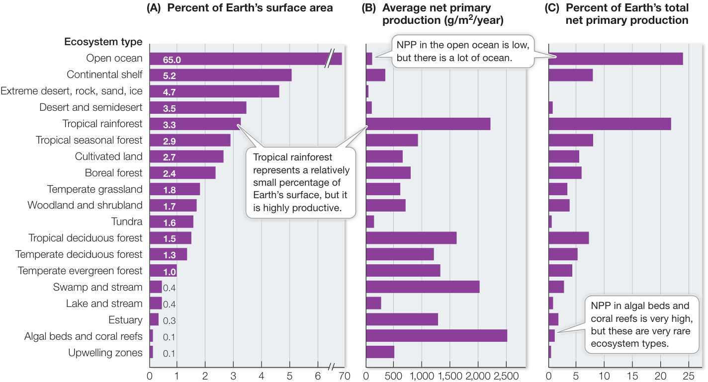
Figure 56.4 Ecosystems Differ in NPP The contribution of different ecosystem types to global NPP can be measured by (A) their geographic extent and (B) their average net primary production. (C) Combining these two measures gives the proportional contribution of each ecosystem type to Earth’s total NPP. (Data primarily based on R. H. Whittaker and G. E. Likens. 1973. Hum Ecol 1: 357–369 and R. H. Whittaker and G. E. Likens. 1975. In Primary Productivity of the Biosphere, H. Lieth and R. H. Whittaker [Eds.], pp. 305–328. Springer-Verlag: New York.)
In addition to being affected by global climate, terrestrial NPP is also affected by nutrient availability and atmospheric CO2 concentrations. How these two factors affect primary production is of special interest given the increasing use of artificial fertilizers and rising atmospheric CO2 concentrations from the burning of fossil fuels (see Key Concept 56.4). A looming question is whether plants, by taking up CO2, might be able to offset increasing CO2 emissions. An ambitious experiment exploring this possibility was conducted in 1996. The FACE (free-air CO2 enrichment) experiment involved artificially increasing CO2 concentrations within arenas constructed around pine trees in North Carolina (Figure 56.6A). To test whether nutrients were a limiting factor, nitrogen was added to half the plots. By late in 2000, trees showed a slight increase in NPP (measured as woody tissue biomass) in the elevated CO2 plots compared with the ambient plots (Figure 56.6B). The increase in NPP, however, was significant only in the fertilized plots, suggesting that nutrients are a limiting factor in the assimilation of CO2 by plants. Since the initial FACE experiment, more than 12 similar large-scale experiments have been conducted in a variety of ecosystems, including grasslands and agricultural crops. The results generally confirm those found in North Carolina, but there are differences. Trees are generally more responsive than herbaceous species to elevated CO2 concentrations, and grain crop yields increase far less than anticipated.
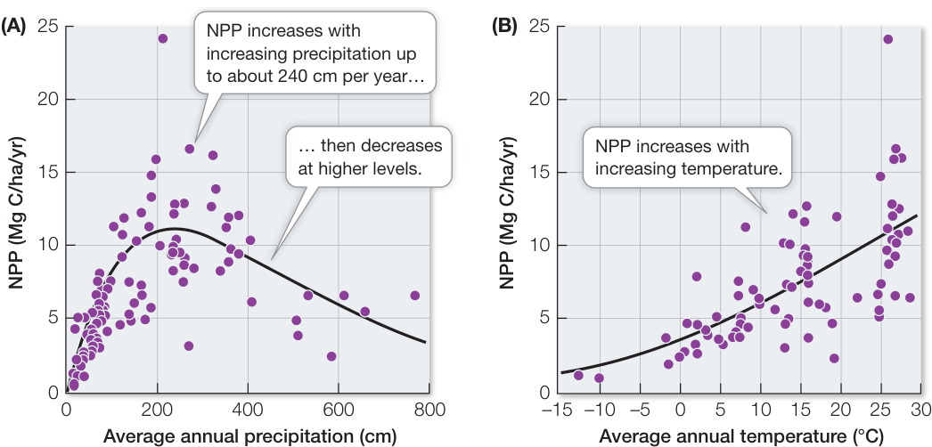
Figure 56.5 Global Patterns of Terrestrial NPP Correlate with Climate The plots show the relationships between NPP for different terrestrial ecosystems and (A) precipitation and (B) temperature of those ecosystems worldwide. (1 megagram or Mg = 106 g.) (After E. A. G. Schuur. 2003. Ecology 84: 1165–1170.)
The FACE experiments remind us that terrestrial ecosystems can vary widely in their NPP, as you saw in Figure 56.4. Clearly some of this variability is a simple consequence of global and regional climate promoting the formation of certain types of ecosystems and biomes, as you saw illustrated by the Walter climate diagrams in Chapter 52. But the types of plant species present can also determine the NPP of an ecosystem. For a given set of environmental conditions, plant species can vary widely in their NPP depending on their photosynthetic pathway (e.g., C3 versus C4 plants, or trees versus shrubs versus grasses), which regulates their rate of photosynthesis. Moreover, nutrient limitation can play a major role in NPP in certain ecosystems. For example, in low-land tropical forests, NPP is often limited by phosphorus, calcium, and potassium. In temperate and arctic ecosystems, nitrogen and phosphorus can be limiting.
Connect the Concepts As discussed in Key Concept 10.4, C3 and C4 plants differ in how they fix CO2 and can be distinguished according to whether the first product of CO2 fixation is a three-or four-carbon molecule (see Figure 10.16).
Light and nutrients combine to control aquatic primary production
Chapter 52 described how Earth’s topography affects water depth, creating gradients in light, temperature, water pressure, and nutrient availability. The main primary producers in aquatic ecosystems—phytoplankton and algae—are most limited by light and nutrients along continental margins (coastal zones) and in the surface waters of oceans and lakes (photic zones) (see Figure 52.9C,D). Oceanic NPP peaks at mid-latitudes and along the continental margins (see Figure 56.3B) because these are regions where nutrient concentrations from ocean upwelling are high. Higher NPP is associated with estuaries as well, where nutrients can be “outwelled” from watershed runoff to coastal zones.
In aquatic systems, NPP is limited primarily by iron, nitrogen, and phosphorus. The relative importance of these three nutrients varies depending on the aquatic ecosystem. In much of the open ocean, NPP is limited primarily by nitrogen. But in some locations, particularly the equatorial Pacific Ocean where excess nitrogen has been detected in surface waters, NPP by phytoplankton may be more limited by iron. In a series of experiments in the mid-1990s, biological oceanographers added iron sulfite to the surface waters off the Galápagos archipelago and in the Southern Ocean to test the hypothesis that oceanic NPP, and thus the potential of the ocean to take up CO2 and combat global warming and ocean acidification (see p. 1270), was limited primarily by iron. The experiments showed that NPP was as much as four-to tenfold higher in the plume of water that received the iron additions. While the experiments show that iron limitation is a major factor in reducing the ability of the ocean to absorb CO2 from the atmosphere, large-scale fertilization of the oceans is impractical at best, and may be somewhat counteracted by respiration of CO2 by zooplankton and bacteria feeding on phytoplankton.
In lake ecosystems, NPP is limited primarily by phosphorus. The effect of phosphorus on lake NPP was first studied in connection with the declining water quality of lakes in North America and Europe. Wastewater and sewage were implicated in a dramatic increase in eutrophication, a process of ecosystem change initiated by an increase in nutrients consumed by phytoplankton, cyanobacteria, and algae in aquatic systems. Eutrophication can result in the explosive growth of algae (algal blooms). Decomposition of large volumes of dead algae by bacteria can in turn severely deplete oxygen needed by aquatic life (hypoxia). To understand which nutrients were most important to the blooms, David Schindler and colleagues conducted whole lake fertilization experiments, starting in 1969, in a set of small lakes in Ontario, Canada. They added nitrogen, carbon, and phosphorus to all or half of several lakes and found that phosphorus was the major trigger for phytoplankton and cyanobacteria blooms (Figure 56.7). These experiments set in motion a campaign to reduce phosphorus in wastewater by recommending the banning of phosphates in detergents and stripping them chemically in sewage treatment plants.
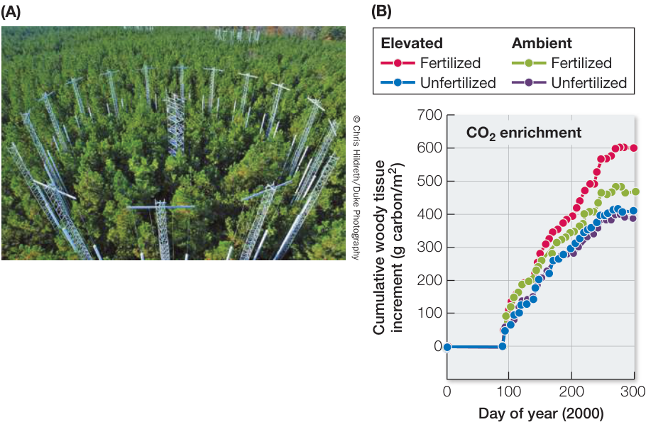
Figure 56.6 FACE Experiment: Effects of CO2 and Nutrients on NPP (A) The free-air CO2 enrichment (FACE) experiment involved releasing CO2 from towers constructed around pine trees. (B) The trees grew better under conditions of elevated CO2 (550 parts per million) and nutrients than they did under ambient conditions. Without added nutrients, elevated CO2 had a minimal effect on tree growth. (After R. Oren et al. 2001. Nature 411: 469–472.)
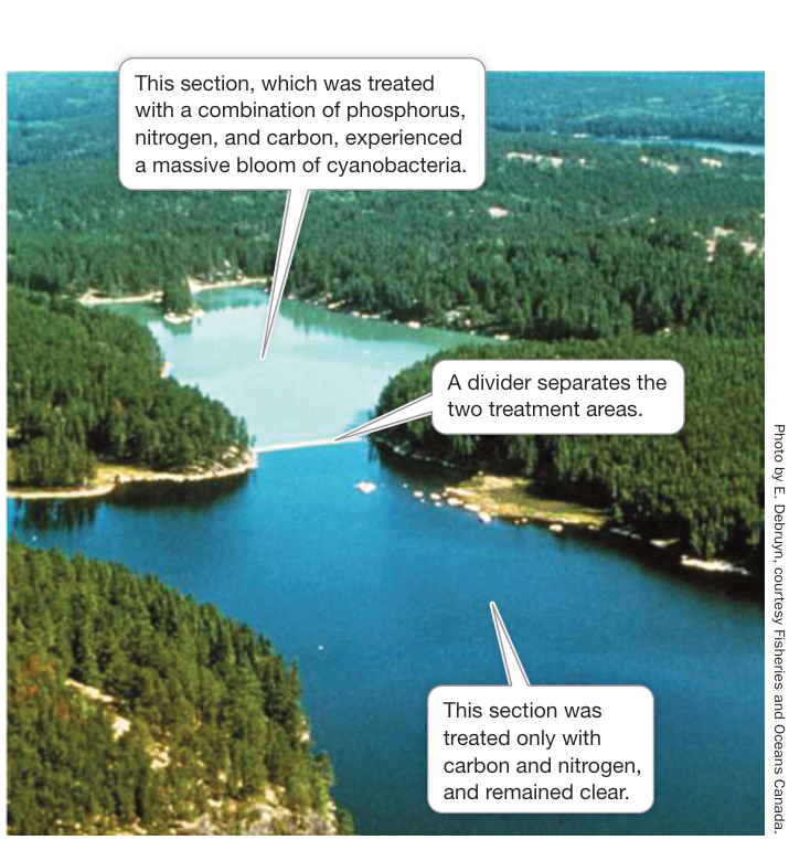
Figure 56.7 Lake NPP Responds to Phosphorus Fertilization Experiments show that the addition of phosphorus to a lake causes massive phytoplankton and cyanobacteria blooms.
Recap and Assess
Fixed carbon, be it from photosynthesis or chemosynthesis, is used to measure primary production. Net primary production is the amount of biomass incorporated into the tissues of primary producers after respiration, and it varies with latitude and ecosystem type. On land, NPP is highest in the tropics where temperatures are high year-round and rainfall is abundant. In the oceans, NPP peaks along continental margins and in areas of upwelling, where the main primary producers—phytoplankton and algae—have access to light and nutrients. Nutrient runoff from agriculture and wastewater can cause eutrophication in aquatic systems, resulting in algal blooms and deadly low oxygen conditions (hypoxia).
- Consider Figure 56.4. How does the average net primary production differ between the open ocean and algal beds and coral reefs? Why, then, does the open ocean account for such a high percentage of Earth’s total NPP?
- Atmospheric CO2 concentrations are rising at unprecedented rates. Is it reasonable to assume that primary producers on land and in the oceans will be able to appreciably lower global CO2 concentrations? What evidence is there to support your answer?
- Describe the process of eutrophication and name the nutrient most responsible for this process in lake systems.
Once the energy captured by primary producers is fixed as NPP, consumption by heterotrophs transfers a fraction of that energy to higher trophic levels. Next we will consider in more detail the factors important to the movement and loss of energy between trophic levels.
Food Webs Transfer Energy
Learning Objectives
- 56.3.1 Describe the factors important in net secondary production, and how production efficiencies differ for ectotherms and endotherms.
- 56.3.2 Discuss why trophic efficiencies are higher in aquatic than in terrestrial ecosystems, and explain how this affects production throughout the food web.
- 56.3.3 Explain why the flow of energy in food webs is influenced by the relative contributions of bottom-up and top-down forces, the number of trophic levels, and the presence of omnivory.
- 56.3.4 Provide hypotheses that explain the factors important to trophic level length.
You know from Chapter 55 that food webs can be constructed to represent the interactions and energy transfers that occur between different species and trophic levels. For example, the food web presented in Figure 55.3 shows the connections among primary producers and consumers in Yellowstone National Park. While the arrows indicate the trophic connections among species, they do not show how much energy is actually being transferred up the food web and converted into secondary production. We will now consider the factors important to secondary production.
Key Concept 8.1 described how, during energy transfer, some energy is lost as “unusable” to the system (second law of thermodynamics) and thus is unavailable to do work. For food webs, the consequence of this loss is that only part of the primary production consumed by heterotrophs is converted into heterotroph biomass. What factors are important to this movement and loss of energy from primary to secondary production? Net secondary production, or the amount of biomass obtained from the consumption of other organisms, depends on how much plant tissue is consumed (consumption efficiency), how much of the consumed food can actually be digested versus released as feces and urine (assimilation efficiency), and how much of the digested food is used in metabolic activities and released as CO2 through respiration versus stored as biomass (production efficiency) (Figure 56.8). We can think of production efficiency as the percentage of energy stored in assimilated food that is used to produce new biomass.
Consumers can vary dramatically in production efficiency. For example, endotherms have much lower production efficiencies than ectotherms (Table 56.1). Because endotherms have to maintain high body temperatures, they have higher metabolic rates than ectotherms, and thus have less energy left over to devote to growth and reproduction. Moreover, endotherms vary in production efficiency depending on body size and metabolism. Larger mammals have lower metabolic rates and higher production efficiencies compared with smaller mammals and birds, whose greater surface area-to-biomass ratios result in more heat loss and higher metabolic rates (see Key Concept 38.5).
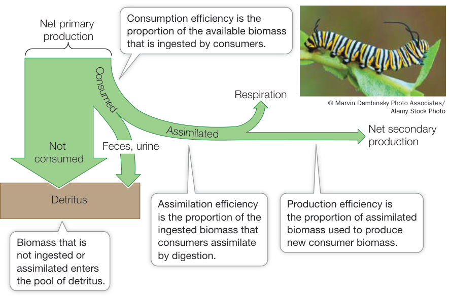
Figure 56.8 Energy Flow and Net Secondary Production in an Herbivore The proportion of energy transferred between a caterpillar and its plant food depends on efficiencies of consumption, assimilation, and production. Q: Why do you think herbivores have lower production efficiencies than carnivores?
Because production efficiency affects the growth and reproduction of consumers, changes in the quality and quantity of food can lead to population declines. Research on Steller sea lions (Eumetopias jubatus) in the Gulf of Alaska and the Aleutian Islands offers a case in point. Sea lion populations declined by 85% over a 25-year period starting in the early 1970s. Surveys of sea lion individuals showed that they were smaller and had lower birth rates compared with individuals before the decline, suggesting that food was a limiting factor. Prior to the decline, sea lions mostly fed on herring, rich in fats, along with lesser amounts of cod and pollock. But when herring populations declined in the 1970s, the sea lion diet consisted mostly of cod and pollock. The energy per gram of biomass of pollock and cod is roughly half that of herring, so sea lions would have needed to eat twice as much pollock and herring to make up for the loss in herring calories. While plenty of fish were available, consumption of a greater percentage of inferior food represented a decline in production efficiency, which in turn translated into a decline in sea lion populations.
The amount of energy transferred within food webs depends on trophic efficiency
In addition to understanding how energy flows between individual consumers, we can also consider how it flows between trophic levels. Trophic efficiency is a measure of the amount of energy at one trophic level divided by the amount of energy at the trophic level immediately below it. Trophic efficiency varies among ecosystems as well as trophic levels. Pyramid diagrams such as those in Figure 56.9 illustrate the proportions of energy transferred from each trophic level to the next, making it possible to compare energy flow in different ecosystems. Pyramid diagrams can also be used to illustrate the amount of biomass found at each trophic level. As seen in Figure 56.9A,B, terrestrial ecosystems progressively lose energy from one trophic level to the next through trophic inefficiencies, especially between the primary producer and primary consumer levels. Note also that terrestrial ecosystems support less biomass at higher trophic levels than at lower trophic levels. Forest ecosystems have lower trophic efficiency than grasslands because much of the biomass in forests is in the form of wood, most of which is unavailable to primary consumers.
In aquatic systems, trophic efficiencies are much higher. Here pyramid diagrams also show a progressive loss of energy at higher trophic levels, as in terrestrial systems, but the corresponding biomass pyramids are inverted (see Figure 56.9C). Why might this be? The phytoplankton that are the primary producers in aquatic ecosystems grow and reproduce much more rapidly than do the zooplankton and small fishes that consume them, so their smaller biomass, with its rapid rate of primary production, can actually support a larger biomass of primary consumers. In part, this difference between terrestrial and aquatic systems explains why land is green but oceans are blue. Terrestrial ecosystems have primary production that far exceeds rates of herbivory,
Table 56.1 Production Efficiencies of Consumers
| Consumer group | Production efficiency (%) |
|---|---|
| ENDOTHERMS | |
| Birds | 1.3 |
| Small mammals | 1.5 |
| Large mammals | 3.1 |
| ECTOTHERMS | |
| Fishes and social insects | 9.8 |
| Nonsocial insects | 40.7 |
| Herbivores | 38.8 |
| Detritivores | 47.0 |
| Carnivores | 55.6 |
| Non-insect invertebrates | 25.0 |
| Herbivores | 20.9 |
| Detritivores | 36.2 |
| Carnivores | 27.6 |
Source: Data from W. F. Humphreys. 1979. J Anim Ecol 48: 427–453.
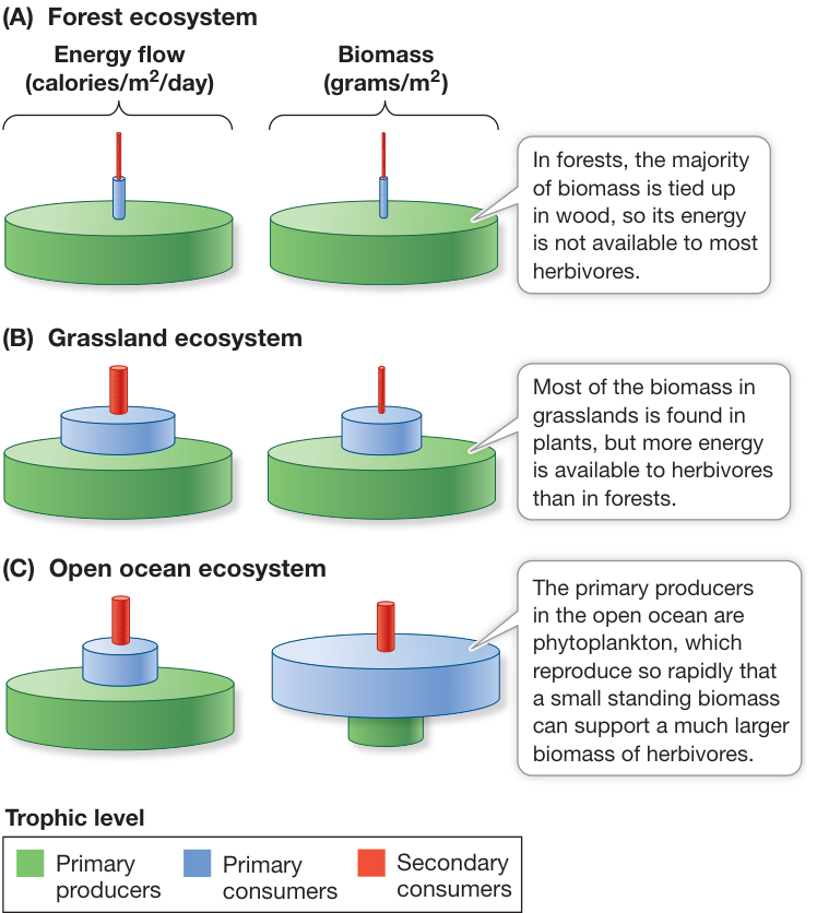
Figure 56.9 Pyramid Diagrams Show Energy Flow and Biomass in Food Webs Pyramid diagrams allow ecologists to compare patterns of energy flow and biomass in food webs. (A) Forest ecosystems have lower trophic efficiency than (B) grasslands because much of the biomass in forests is wood, and thus unavailable to most primary consumers. (C) In open oceans, the rapid rate of primary production can support a larger biomass of primary consumers.
while the opposite is true for large portions of the ocean. Overall, estimates suggest that, on average, only 13% of terrestrial biomass is consumed by primary consumers, compared with 35% in aquatic ecosystems.
Food webs are controlled by bottom-up and top-down forces
The control of energy flow in an ecosystem occurs in two ways. First, as we discussed in Key Concept 56.2, the amount of energy entering a food web can depend on the NPP of that system, which depends on such factors as rainfall, temperature, light, and nutrients. The more NPP entering the system, the more energy that is passed up the food web to consumers. This flow of energy is referred to as “bottom-up” control because it comes from the “bottom,” or primary producer trophic level (Figure 56.10A). The other type of control on energy flow can come from consumers at higher trophic levels, who regulate the amount of NPP by feeding on lower trophic levels. This control is referred to as “top-down” control because it comes from the “top,” or the secondary consumer trophic level.
All food webs are controlled by both bottom-up and top-down pathways, but the relative importance of that control can vary depending on the food web in question. For example, food webs that experience a trophic cascade driven by a key-stone predator, as you saw in the examples of gray wolves (Canis lupus) in Yellowstone National Park (see Figure 55.9) and sea otters (Enhydra lutris) in kelp forests, are dominated by top-down control (see Key Concept 55.3). In those two cases, it was the top predator that controlled the prevalence of primary producers (aspen and kelp, respectively), rather than limiting resources per se.
There are also clear examples of bottom-up control in food webs. For example, in a study of pelagic ecosystems off the coast of western North America, researchers found a strong positive correlation between phytoplankton abundance, zooplankton abundance, and fish production (measured from fisheries-catch data). Phytoplankton abundance in this region is largely controlled by ocean upwelling, which brings nutrients to the light-saturated surface waters for use by phytoplankton. The intensity of upwelling varies along the coast, thus creating “hotspots” of productivity that are reflected in the fish populations of the region.
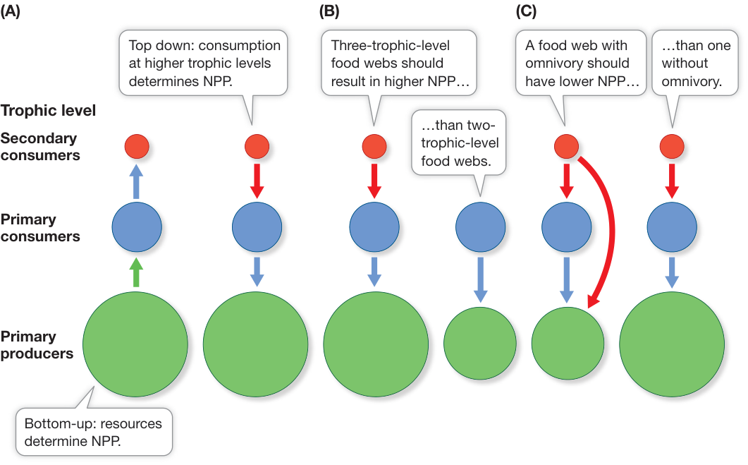
Figure 56.10 Bottom-up and Top-down Control of Food Webs (A) Production in an ecosystem can be viewed as mostly being controlled by limiting resources (bottom-up) or by consumers at higher trophic levels (top-down). (B) A three-level food web, in which the secondary consumer affects the primary consumer’s abundance, has higher NPP (represented by the size of the green circle) than a two- or four-level food web. (C) A three-level food web with omnivory has lower NPP than a food web without omnivory.
The number of trophic levels can control the flow of energy through food webs
In the previous section we learned that changes in the abundance of organisms at one trophic level can influence the energy flow at multiple trophic levels. You might imagine that the number of trophic levels in a food web could be important in the magnitude of that influence. Indeed, all things being equal, a three-level food web, in which the secondary consumer affects the primary consumer’s abundance, should have higher NPP than a two-or four-level food web in which primary consumers have less secondary consumer control (Figure 56.10B). Omnivory, or feeding on more than one trophic level, can also change the way energy is transferred in food webs by essentially “collapsing” trophic levels on one another. For example, a three-level food web with a secondary consumer feeding on both the primary consumer and primary producer should have lower NPP than a three-level food web without omnivory (Figure 56.10C). That’s because even though the secondary consumer indirectly benefits the primary producer by feeding at the primary consumer level, it partially negates this effect by directly feeding on the primary producer as well.
While the number of trophic levels in foods webs can vary, most food webs have three or four trophic levels, with the rare exception of five or more in some systems. What factors might be important in limiting the number of trophic levels in food webs? Several factors have been hypothesized to be important:
- The amount of NPP entering the system: This hypothesis suggests that bottom-up factors can influence trophic structure. Given that a large amount of energy is lost from one trophic level to the next (see Figure 56.9), the number of trophic levels will be limited by the amount of energy that can sustain populations at higher trophic levels.
- The amount of disturbance: This hypothesis suggests that longer food webs are less likely to recover from disturbances than shorter food webs, which can presumably reassemble more quickly given the fewer trophic levels, and species, involved.
- The evolutionary constraints on top predators: This hypothesis focuses on the idea that no organisms on Earth today, with the exception of humans, have evolved to capture apex predators such as birds of prey, sharks, orcas (Orcinus orca), and polar bears (Ursus maritimus). With evolutionary constraints maintaining top predators at the pinnacle of food webs, the number of higher trophic levels is limited.
Recap and Assess
Once energy captured by primary producers is fixed as NPP, consumption by heterotrophs transfers a fraction of that energy to higher trophic levels (net secondary production). Terrestrial systems have lower trophic efficiencies than aquatic systems, where the rapid rate of primary production supports greater secondary production. The flow of energy in food webs is influenced by the relative contribution of bottom-up and top-down forces, the number of trophic levels, and the presence of omnivory. Food webs are typically restricted to three or four trophic levels because of energy limitations at higher trophic levels, the effects of disturbance, and/or evolutionary constraints on top predators.
- Suppose there are two food webs, one in a forest and the other in a lake. All else being equal, which food web would have the higher trophic efficiency, and why? Comparing different species, which would have the higher production efficiency, a bear or a crayfish? Explain your answer.
- Now compare two food webs in different lakes. One has three trophic levels, and the other has four. All else being equal, which would have the higher NPP? Why? If you added omnivory to the top level of the food web with four trophic levels, how would it differ in NPP compared with the food web without omnivory?
- Compare a tropical rainforest food web that has five trophic levels with a desert food web having three trophic levels. What hypothesis might best explain the difference in trophic level length between the two ecosystems?
We’ve considered how energy flows from primary producers to consumers, and the implications of that flow for food webs. Besides energy, a key component of the metabolism and growth of organisms is nutrients (including water). Earlier in the chapter you read that nutrients continually cycle between living organisms and the abiotic environment via nutrient cycling (see Figure 56.1C). We will consider nutrient cycling next.
56.4
Nutrient Cycling in Ecosystems
Nutrient Cycling in Ecosystems
Biological Transformations
Learning Objectives
- 56.4.1 Define biogeochemical cycles and understand decomposition and mineralization in nutrient cycling.
- 56.4.2 Discuss the hydrologic cycle, including residence times of water molecules.
- 56.4.3 Describe Earth’s carbon cycle and how burning fossil fuels is changing Earth’s climate and oceans.
- 56.4.4 Explain the basics, and the relative roles of microbes versus geological processes, in the nitrogen, phosphorus, and sulfur cycles.
All nutrients that make up the tissues of organisms originate from either soil, water, or the atmosphere, and then cycle between organisms and their environment through (1) primary and secondary production and (2) decomposition (Figure 56.11). We considered production in the last two key concepts, but not decomposition. Decomposition occurs when detritus, or dead organisms and
Nutrient Cycling in Ecosystems
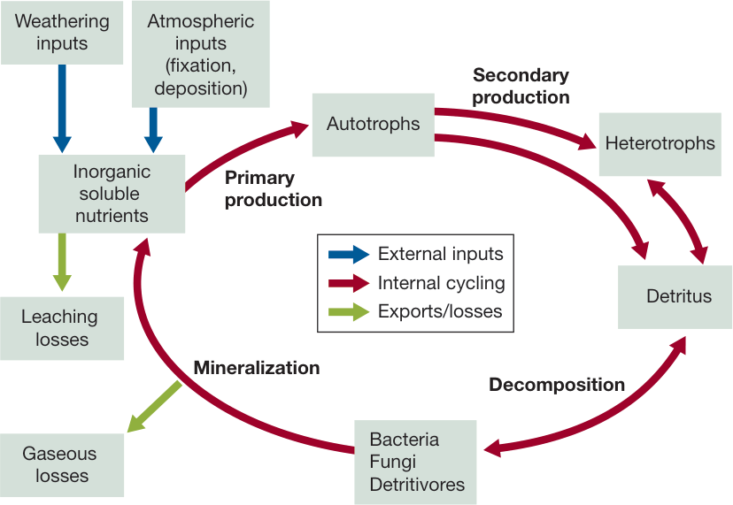
Figure 56.11 Nutrient Cycles A generalized nutrient cycle, showing the movement of nutrients among biotic and abiotic compartments of an ecosystem and the potential pathways for inputs and losses.
Because geological, chemical, and biological processes are all important in moving materials around the planet, the pattern of movement of an element is called its biogeochemical cycle. The cycles are considered in terms of pools—the amount of elements within certain parts of the abiotic and biotic environment—and fluxes, or the rates of movement between pools. We will consider the biogeochemical cycling of water, carbon, nitrogen, phosphorus, and sulfur at the global scale because of their functional roles in biological systems and their roles as pollutants in the environment.
Water cycles rapidly around the globe
We start our discussion of global biogeochemical cycles with the water cycle—known as the hydrologic cycle—not only because water serves as an essential element for organisms but because it plays an important role in transporting nutrients between compartments (Figure 56.12). Energy from the Sun drives the hydrologic cycle by evaporating water from the vast surfaces of the oceans. Most of the water is returned to the oceans as rainfall, but a smaller fraction is transported their waste products, are broken down by bacteria and fungi into energy and nutrients. Decomposition releases nutrients in a soluble form that can then be taken up by primary producers and microorganisms. Detritus can come in many forms, including plants and animals, but is mostly made up of plant or algal matter. Detritus must first be broken down into smaller fragments by detritivores such as worms and arthropods before it can undergo mineralization (see Figure 56.11). Mineralization is the process by which animals, bacteria, and fungi convert organic compounds into inorganic soluble nutrients. Along the way, some of the nutrients may be lost to the system as gas to the atmosphere or minerals to ground water. The nutrient cycle is complete when the inorganic soluble nutrients produced through mineralization are used once again by primary producers or bacteria.
The movement of nutrients through food webs from uptake to decomposition—that is, through the biotic components of ecosystems—occurs primarily on a local scale. In contrast, abiotic processes can move nutrients far beyond the boundaries of the local ecosystem. Each of the chemical elements that organisms use in large quantities cycles in a distinctive way through the globe.
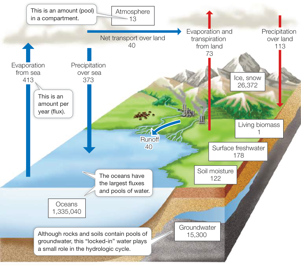
Figure 56.12 The Global Hydrologic Cycle Water is essential for life on Earth. The estimated pools in major compartments (white boxes) and the annual fluxes between compartments (arrows) are expressed in units of grams. (After K. E. Trenberth et al. 2007. J Hydrometeor 8: 758–769; F. S. Chapin et al. 2002. Principles of Terrestrial Ecosystem Ecology, p. 351. Springer-Verlag: New York.)
over land. Ocean water vapor combines with terrestrial water vapor from soils, lakes and rivers, and plants as a consequence of evapotranspiration, and falls as precipitation over land. Terrestrial precipitation eventually returns to the oceans via streams, coastal runoff, and groundwater flows. More than half of this volume of water is carried back to the oceans by Earth’s four largest rivers: the Amazon in South America, the Nile in Africa, the Mississippi in North America, and the Yangtze in Asia.
Connect the Concepts In Key Concept 52.3, evapotranspiration is defined as the evaporative transfer of heat and water from the surfaces of plants into the atmosphere, which reduces air temperature and increases moisture.
Despite their relatively small volume, rivers play a disproportionate role in the hydrologic cycle because the average residence time of a water molecule in rivers is only a few years. By comparison, the average residence time of a water molecule in lakes ranges from a few years to centuries. The larger the lake, the longer the residence time; the residence time for water in the top portion of Lake Superior, for example, is 1,500–2,000 years, and the water at the bottom of this massive lake cycles over much longer time scales. In the oceans the average residence time of a water molecule is about 3,000 years. Other pools of water include glaciers (with residence times of 20–100 years), seasonal snow cover (a few months), and soil moisture (1–2 months). The average residence time of water in the bodies of organisms is particularly brief, averaging just under a week.
Although large amounts of groundwater are present in underground pools called aquifers, this water has a long residence time underground and plays only a small role in the hydrologic cycle. In some places, however, aquifers are being depleted because humans are using groundwater more rapidly than it can be replaced, primarily for irrigation. On the North China Plain, depletion of shallow aquifers is forcing people to sink wells more than 1,000 meters deep to reach groundwater. If current water consumption patterns continue, it has been estimated that by 2025 at least 48% of the current world population will live in areas with inadequate water supplies.
The carbon cycle is being altered by human activities, resulting in climate change
All of the important macromolecules that make up living organisms contain carbon, and much of the energy that organisms use to fuel their metabolic activities is stored in carbon-containing (organic) compounds. On land, biological processes move carbon directly between organisms and the atmosphere as terrestrial organisms take up carbon during photosynthesis and return it to the atmosphere through respiration and metabolism (Figure 56.13). In contrast,
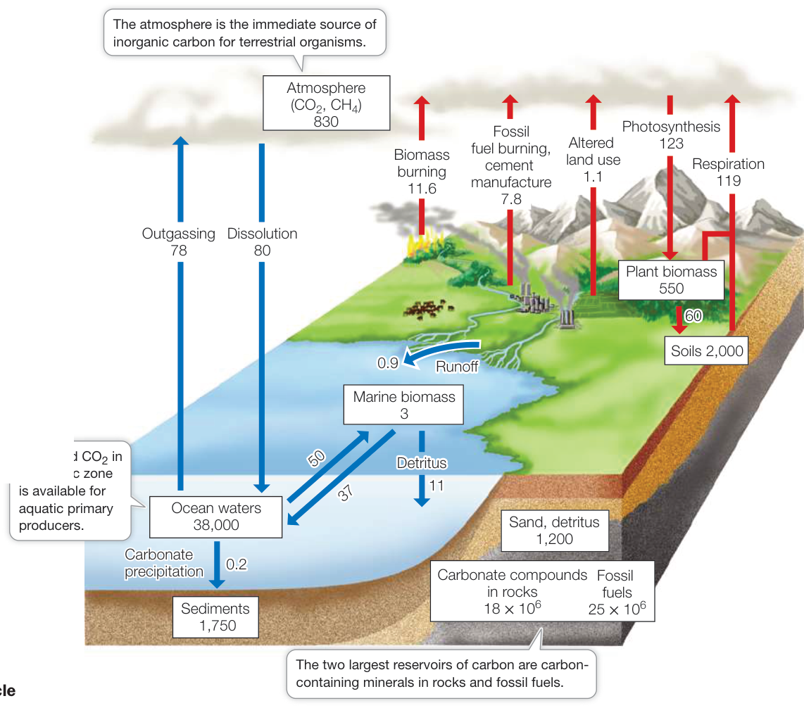
Figure 56.13 The Global Carbon Cycle Carbon is the basis of the organic molecules and energy essential for life. The estimated pools in major compartments (white boxes) and the annual fluxes between compartments (arrows) are expressed in units of grams. (After P. Ciais et al. 2013. In Climate Change 2013: The Physical Science Basis. Contribution of Working Group I to the Fifth Assessment Report of the Intergovernmental Panel on Climate Change, T. F. Stocker et al. [Eds.], pp. 466–570, Cambridge University Press, Cambridge, UK and New York, NY, USA; W. H. Schlesinger and E. S. Bernhardt. 2013. In Biogeochemistry: An Analysis of Global Change 3rd ed. W. H. Schlesinger and E. S. Bernhardt [Eds.], pp. 445–467. Academic Press: Cambridge, MA; F. S. Chapin et al. 2002. Principles of Terrestrial Ecosystem Ecology, p. 336. Springer-Verlag: New York.)
Animation 56.2 The Global Carbon Cycle carbon dioxide moves into ocean waters from the atmosphere primarily by simple diffusion at the ocean surface; this dissolved CO2 is the source of the carbon used by marine primary producers. Even taken together, however, the amounts of carbon in the atmosphere, in soils, and in living and dead organisms are dwarfed by the vast quantities of carbon stored in terrestrial rocks, in fossil fuels, in marine sediments, and in seawater in the form of carbonate ions (CO3-2) or bicarbonate ions (HCO3-) (see Figure 56.13).
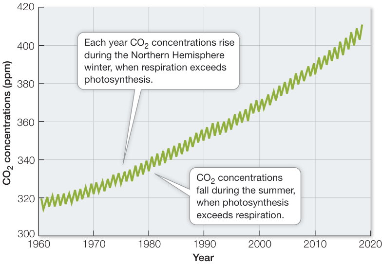
Figure 56.14 Atmospheric CO2 Concentrations Are Increasing Carbon dioxide concentrations have been recorded since 1960 on top of Mauna Loa, Hawaii, far from most sources of human-generated CO2 emissions. Although concentrations vary seasonally, the trend has been consistently upward. (After C. D. Keeling et al. 2001. I. Global aspects, SIO Reference Series, No. 01–06. Scripps Institution of Oceanography. San Diego. Last updated June 2019.) Media Clip 56.1 Time-Lapse of Global CO2 Emissions Life12e.com/mc56.1
Over the span of life’s existence on Earth, quantities of carbon were removed from active cycling when organisms died in large numbers and were buried in sediments lacking oxygen. In such anaerobic environments, with few detritivores to reduce organic carbon to CO2, organic molecules accumulate and are eventually transformed into deposits of oil, natural gas, coal, or peat—the fossil fuels that modern humans use as a combustible source of energy. Humans have discovered and used these fossil fuels at ever-increasing rates during the past 150 years. As a result, CO2, one of the final products of burning fossil fuels, is being released into the atmosphere faster than it is absorbed in the oceans or incorporated into terrestrial biomass. Measurements of CO2 on the top of Mauna Loa, Hawaii, show that, even though atmospheric CO2 varies seasonally because of the change in NPP, it has steadily increased over the last 60 years of data collection (Figure 56.14).
ATMOSPHERIC CO2 AND GLOBAL CLIMATE CHANGE Carbon dioxide is a greenhouse gas, so we would expect increasing atmospheric CO2 concentrations to trap more heat in Earth’s atmosphere and raise temperatures at Earth’s surface (see Figure 52.2). What evidence do we have that this is occurring? Measurements of gases in air trapped in the Antarctic and Greenland ice caps show that temperatures have been warmer when atmospheric CO2 concentrations have been higher and cooler when they have been lower (Figure 56.15). For example, the atmospheric CO2 concentration was very low at the end of the last glaciation (180 parts per million [ppm]), 18,000 years ago, when temperatures were much colder than they are today. In contrast, during a warm interval between 11,000 years ago and the start of the Industrial Revolution (1750), the concentration of CO2 in Earth’s atmosphere was between 260 ppm and 280 ppm. In 2019, atmospheric CO2 concentration is just over 414 ppm (see Figure 56.14), the highest recorded in the last 800,000 years. The increase in CO2 (and two other greenhouse gases, CH4 and N2O) from the burning of fossil fuels has resulted in a roughly 1-degree Celsius (1.8-degree Fahrenheit) rise in global temperatures compared with those from 1981 to 2010 (a comparison known as a “temperature anomaly”).
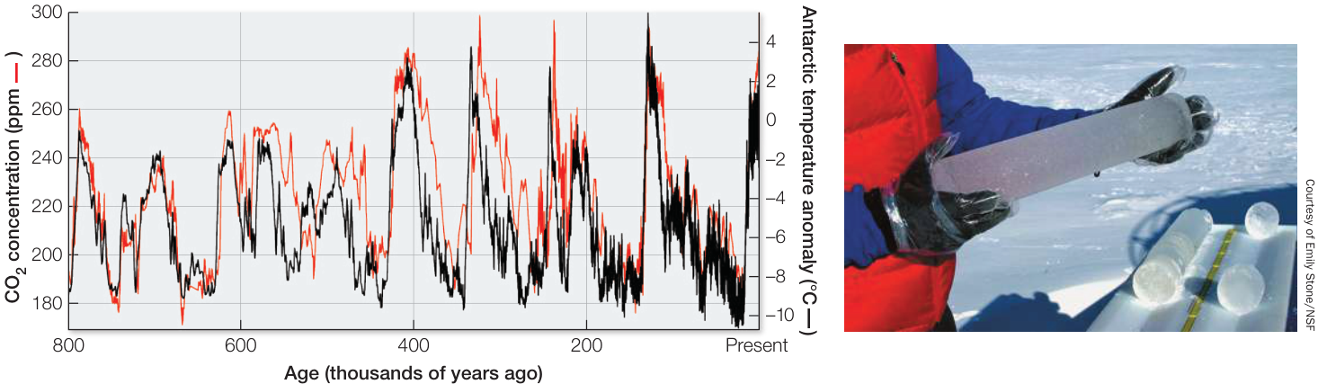
Figure 56.15 Higher Atmospheric CO2 Concentrations Correlate with Warmer Temperatures Atmospheric concentrations of CO2 (measured in air bubbles trapped in Antarctic ice) have varied with temperatures over Antarctica (estimated with oxygen isotope analysis) for more than 800,000 years. “Temperature anomaly” is the change in Antarctic temperatures compared with modern temperatures. (After D. Lüthi et al. 2008. Nature 453: 379–382.)
How global climates and ecosystems will change in response to this rapid warming is a subject of intense investigation. Global warming has already resulted in the shrinking of Arctic sea ice, which is currently the lowest ever recorded. As temperatures continue to rise and glacial ice melts, sea level rises (because of both thermal expansion of ocean waters and the addition of glacial meltwater), increasing flooding of coastal cities and agricultural lands, especially during extreme storm events. Nearly one-third of the world’s population lives in coastal regions, which make up only 4% of Earth’s total land area.
Even though atmospheric is increasing as the result of burning fossil fuels, less than half of the released into the atmosphere by human activities remains in the atmosphere. Where does the rest of the wind up? Much of it is absorbed by the oceans in inorganic forms. Over decades to centuries, the oceans exert a large influence over atmospheric concentrations. Of the absorbed by the ocean, some is used in photosynthesis by phytoplankton in the surface waters. These organisms remove dissolved from water, thereby increasing the rate at which atmospheric is absorbed by surface waters, but as you saw earlier, there are limits to this absorption given nutrient limitation in vast parts of the open ocean. In addition, many marine organisms (including clams, oysters, corals, and planktonic foraminiferans) incorporate carbon in their shells and other structures in the form of calcium carbonate (), which is synthesized by combining bicarbonate ions () and calcium ions () dissolved in seawater. When these organisms die, those shells and their embedded carbon sink to the ocean floor.
Today’s oceans absorb millions of tons of from the atmosphere each day—more than at any time during the past 20 million years. As a result, water near the ocean surface is becoming more acidic. As concentrations in the atmosphere rise, more of the gas diffuses into the water at the ocean surface, where it reacts with water to form carbonic acid (). As levels of carbonic acid rise, the pH of seawater drops. This increase in acidity can have negative effects on many marine organisms, particularly corals. The combination of decreasing pH and increasing water temperature to which corals are being exposed results in coral bleaching and sometimes the death of corals. Because so many other reef species depend on corals and the structure they provide, an entire reef community can collapse if its corals fail to thrive.
Connect the Concepts As described in Investigating Life: Corals in Hot Water in Chapter 1, coral bleaching occurs when corals are exposed to warm and/or acidic waters, causing expulsion of their photosynthetic algal symbionts.
But as you read in the opening story, the effects of and ocean acidification vary depending on the organisms or ecosystems considered. Investigating Life: Food Webs in an Acidic and Warming Ocean describes research in Sweden by marine ecologists interested in the effects of ocean acidification and warming on an ecologically critical but predominantly primary-producer-dominated ecosystem: estuaries. In this system, the researchers focused on benthic microalgae, an important food source for a diversity of sediment-dwelling herbivores, including crustaceans, snails, and worms. Benthic microalgae indirectly benefit from higher trophic levels, particularly omnivores that feed on macroalgae competitors and herbivores of the microalgae. Using experimental manipulations, the researchers discovered that the biomass of benthic microalgae did not appreciably change under elevated and warming manipulations. As it turned out, the consumers mediated the effects of ocean acidification and warming on benthic microalgae, suggesting that consumers, or other strongly interacting species in food webs, have the potential to modulate the effects of climate change in complicated and unpredictable ways.
In terrestrial ecosystems, photosynthesis, principally in tropical forests, typically absorbs about the same amount of carbon that is released by terrestrial plants, microbes, and animals through metabolism. In more recent times, as atmospheric increases, the photosynthetic consumption of exceeds its metabolic production, which means Earth’s terrestrial vegetation is storing carbon that would otherwise be increasing atmospheric concentrations—but as we saw in the FACE experiment, we cannot count on terrestrial vegetation to store the vast amounts of excess that human activities produce. Furthermore, climate warming (another result of increasing atmospheric concentrations, as you have already seen) increases plant metabolism and is thus likely to increase the flux of from vegetation into the atmosphere.
The nitrogen cycle is dominated by biotic processes
Nitrogen gas is the most abundant gas in Earth’s atmosphere, but most organisms cannot use nitrogen in its gaseous form. Nitrogen enters the system as atmospheric and is fixed by bacteria into ammonia () (Figure 56.16). Ammonia is rapidly transformed into ammonium (), which can then be used by plants and bacteria. Nitrifying bacteria can transform ammonium to nitrite () and then nitrate (), both forms of nitrogen that plants and bacteria can use. Denitrifying bacteria take nitrate and convert it back to and gases, which are then released back into the atmosphere. Along the way, plants and bacteria incorporate the nitrogen into their tissues, making it available to higher trophic levels as secondary production and eventually to decomposers. Collectively this microbial processing of nitrogen accounts for about 95% of all natural nitrogen flux on Earth, making it a mostly biologically driven cycle (Figure 56.17).
All living organisms require nitrogen, and the inability of the vast majority of organisms to use means that usable nitrogen is often in short supply. Populations of nitrogen-fixing organisms rarely increase in abundance to the extent that nitrogen is no longer limiting, because the end products of their nitrogen fixation are rapidly lost from ecosystems (ammonia by vaporization and denitrification; and nitrate, which is highly water-soluble, by leaching).
Human activities that fix nitrogen, such as the manufacture of artificial fertilizers, have had large and unanticipated effects on the nitrogen cycle. The extensive use of artificial fertilizers on agricultural crops, coupled with the burning of fossil fuels (which generates nitric oxide and nitrogen dioxide), has resulted in total nitrogen fixation by humans being nearly equal to global natural nitrogen fixation (see Figure 56.17). This human-generated
Investigating Life: Food Webs in an Acidic and Warming Ocean
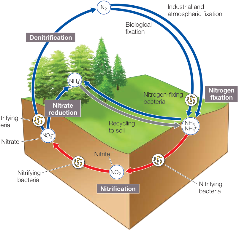
Figure 56.16 The Nitrogen Cycle Nitrogen fixation, nitrification, nitrate reduction, and denitrification are components of an essential chemical cycle that coverts atmospheric nitrogen gas into ammonium ions and nitrate ions—forms of nitrogen that can be taken up by plants—and returns to the atmosphere.
nitrogen flux has been increasing over the past half-century and is expected to continue to increase.
Experiment
Original Paper: C. Alsterberg et al. 2013. Consumers mediate the effects of experimental ocean acidification and warming on primary producers. Proc Natl Acad Sci USA 110: 8603–8608.
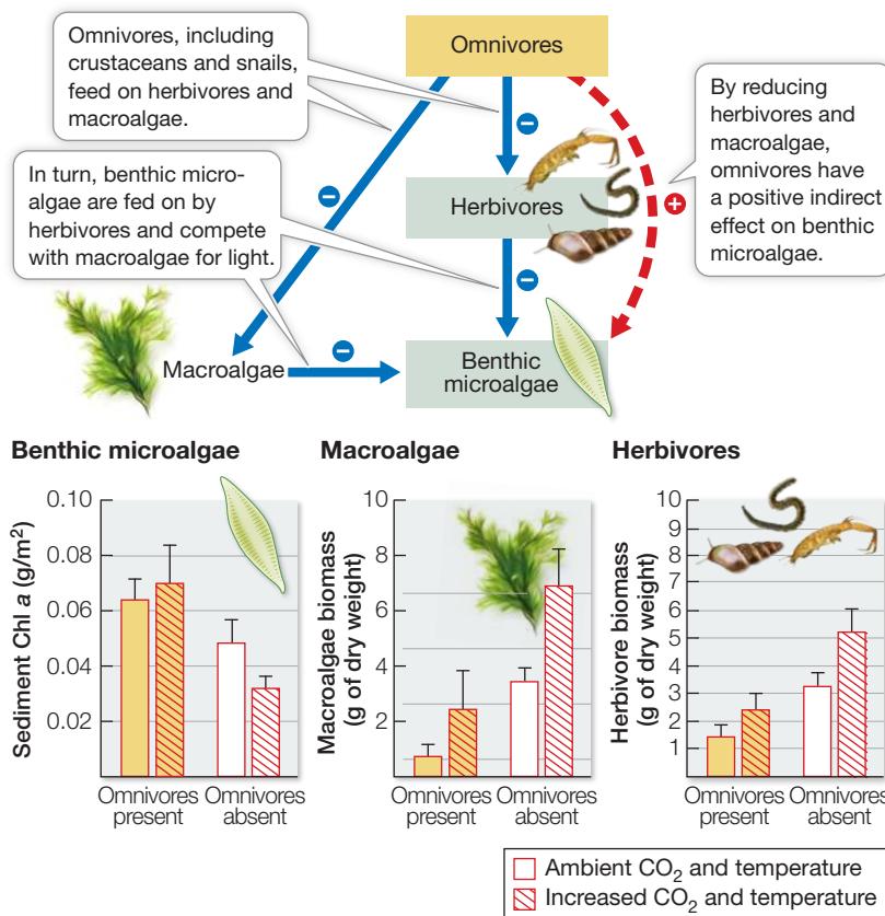
Christian Alsterberg and his colleagues considered how the food web in an estuarine ecosystem on the western coast of Sweden was influenced by ocean acidification and warming. The researchers chose to focus on benthic microalgae (single-celled algae) and their interactions with macroalgae and consumers. In this system, omnivores (i.e., a guild of medium-sized crustaceans and snails that feed on two trophic levels) affect the productivity of benthic microalgae in two ways: (1) they increase the light available to microalgae by feeding on macroalgae, and (2) they prey on herbivores of microalgae (i.e., a guild of small crustaceans, snails, and worms). To estimate the importance of ocean acidification and increased warming in a multispecies food web, the researchers conducted an experiment on the estuarine community in which , temperature, and omnivores were manipulated.
HYPOTHESIS Increasing and temperature will increase the biomass of macroalgae competitors, causing a decline in the biomass of benthic microalgae.
METHOD
- Fill 30-liter buckets with seawater and add microalgae, macroalgae, and herbivores.
- Apply three treatments:
- two levels of seawater temperature (ambient and increased)
- two levels of (ambient and increased)
- two levels of omnivores (present and absent)
- At the end of a 5-week period over the summer, measure the biomass of benthic microalgae (as Chl a concentrations), macroalgae, and herbivores.
RESULTS To simplify, the results (means SEs) from the following treatments are presented: ambient and temperature and increased and temperature, each with and without omnivores
The researchers found that benthic microalgae biomass did not change under increased and temperature. This was true regardless of whether omnivores were present. However, the removal of omnivores did cause a decline in benthic microalgae under ambient conditions, as would be predicted from the food web shown here.
Omnivore removal caused an increase in the biomass of macroalgae competitors and herbivores, which then led to a decline in benthic microalgae. Interestingly, even though there was no effect of increased and temperature on microalgae biomass, the results showed that both macroalgae and herbivores increased in biomass under these conditions compared with under ambient conditions. This was especially the case when omnivores were removed.
CONCLUSION What can you conclude about the effects of increased and temperature on benthic microalgae in this estuarine food web? Explore this question in the following Work with the Data.
Work with the Data
To interpret the Alsterberg et al. study, we consider why benthic microalgae biomass did not change under increased and temperature within the context of the experimental manipulation of the food web.
QUESTIONS
- Draw two food webs for this system, one with and one without the omnivores. Use arrows to indicate the direct (solid) and indirect (dashed) interactions and symbols to indicate negative (-) or positive (+) interactions.
- Now, using data from the graphs in the experiment, modify the two food webs to show how increased and temperature will affect the strength and direction of the food web interactions.
Vary the width of the arrows to indicate the relative strength of the interactions, and use symbols to indicate whether the interactions are negative (-) or positive (+). Indicate in writing whether benthic microalgae increase, decrease, or stay the same compared with under ambient conditions.
- Using the food webs you drew for Question 2, explain why increased and temperature had no effect on microalgae biomass compared with the ambient conditions.
- Under increased and temperature, what would happen to benthic microalgae biomass if the omnivores ceased feeding on macroalgae and just preyed on herbivores?
One consequence of artificial fertilizer production is an increase in the greenhouse gas nitrous oxide (), resulting in more tropospheric ozone () and smog. Tropospheric ozone is itself a greenhouse gas and thus can contribute to global climate change.
Some of the nitrous oxide that enters the atmosphere falls back to land in precipitation or as dry particles. This deposition of nitrogen from the atmosphere has increased dramatically during recent decades. Nitrogen deposition could affect the composition of terrestrial vegetation by favoring those plant species that are best adapted to take advantage of high nutrient levels, and which may then outcompete other species.
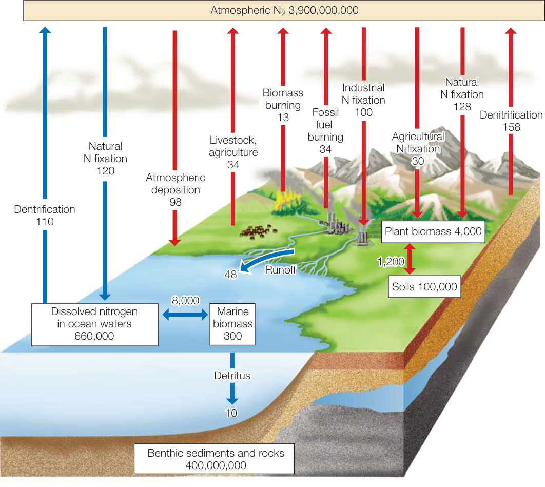
Figure 56.17 The Global Nitrogen Cycle The largest pool of nitrogen is in the atmosphere in the form of nitrogen gas, . Nitrogen cycles through the biosphere primarily via the processes of nitrogen fixation, which converts inorganic nitrogen to an organic form usable by plants, and denitrification, which returns to the atmosphere. The estimated pools in major compartments (white boxes) and the annual fluxes between compartments (arrows) are expressed in units of grams. (Data from J. N. Galloway et al. 2004. Biogeochemistry 70: 153–226; C. C. Cleveland et al. 1999. Global Biogeochem Cycles 13: 623–645; Illustration after F. S. Chapin et al. 2002. Principles of Terrestrial Ecosystem Ecology, p. 344. Springer-Verlag: New York.) Q: How does the industrial fixation of nitrogen (as a percentage) compare with the other forms of fixation on land?
Another consequence of nitrogen fertilizers is eutrophication, a process we considered in Key Concept 56.2 for phosphorus additions in lake ecosystems. In this case, when more nitrogen fertilizer is applied to agricultural lands than can be taken up by the crops, the excess nitrogen moves out of the system in surface runoff, or downward into groundwater, and ultimately ends up in rivers, lakes, and oceans. So-called dead zones have formed near the mouth of the Mississippi River in the Gulf of Mexico as a result of the drainage from interior agricultural fields carrying high concentrations of nitrogen fertilizer.
The global phosphorus cycle is dominated by geochemical processes
Phosphorus accounts for only about 0.1% of Earth’s crust, but it is an essential nutrient for all life forms. It is a key component of cell membranes, DNA, RNA, and ATP. Unlike the other biogeochemical cycles discussed thus far, the phosphorus cycle does not have a significant atmospheric component, although some phosphorus is transported by dust particles. Most of Earth’s phosphorus is in the form of phosphate in rocks and deep-sea sediments, and it cycles very slowly through the geological system because it requires sedimentary rock formation, uplift, and weathering. In contrast, phosphorus in organisms cycles rapidly, and it is often a limiting factor for their growth, particularly for plants. As you learned in Key Concept 56.2, runoff of phosphorus from fertilizers and detergents into aquatic systems can result in eutrophication.
The burning of fossil fuels affects the sulfur cycle
Sulfur is required by all organisms because it is critical in the production of proteins and lignin. Most of Earth’s sulfur supply is locked up in rocks on land and as sulfate salts in deep-sea sediments, but sulfur moves to the atmosphere in a variety of ways. Roughly 10%–20% of atmospheric sulfur is produced in volcanic eruptions. In terrestrial systems, when sulfur in the soil comes in contact with atmospheric oxygen, it is converted to sulfate salts, which can be taken up by plants and eventually incorporated into their tissue. This sulfur ultimately is returned to the atmosphere as via microbial decomposition. In marine systems, many phytoplankton and seaweeds manufacture large quantities of a sulfur-containing compound (dimethylsulfoniopropionate, or DMSP) to maintain their salt and water balance. When broken down, DMSP releases dimethyl sulfide (), the principal odorant of rotting seaweed. Because the quantities of phytoplankton in the oceans are enormous, dimethyl sulfide production accounts for about half of the biotic component of the global sulfur cycle.
Atmospheric sulfur exists in gaseous and particulate forms and plays an important role in global climate. Cloud formation is dependent on small particles around which water can condense. Dimethyl sulfide is a major component of such particles, so increases in atmospheric sulfur concentrations increase cloud cover and reduce the amount of incoming solar radiation, affecting Earth’s temperature. In addition, and produced by humans from the burning of coal and oil react with water molecules in the atmosphere to form sulfuric acid () and nitric acid (), respectively. These acids can travel hundreds of kilometers in the atmosphere before they are released as acid rain. Acid rain can damage forests and lakes, affecting the food webs they support. Restriction on the emissions of sulfur in North America and Europe has resulted in significant reductions in acid rain. Research shows that once acidity is reduced, forest and aquatic systems can quickly recover. Acid rain remains a problem in some countries such as China and India, where rapid industrialization and the lack of restrictions create high sulfur emissions.
Recap and Assess
Nutrient cycling in ecosystems and global biogeochemical cycles involves chemical and biological transformations through production, decomposition, and mineralization. The hydrologic cycle is not only crucial in making water available to organisms but also in transporting nutrients within ecosystems. Carbon moves through biological systems and returns to the atmosphere through respiration. Burning of fossil fuels increases the carbon dioxide and sulfur in the atmosphere, which is implicated in global warming and acidic conditions in lakes and oceans. The nitrogen cycle is dominated by biotic transformations controlled by bacteria, whereas phosphorus and sulfur cycles are dominated by geochemical processes.
- The residence time of a water molecule is short in organisms, soil, and rivers and is much longer in lakes, glaciers, and oceans. Why?
- Why is the concentration of rising in the atmosphere and oceans? How does this rise in affect climate and ocean chemistry?
- Explain how the nitrogen cycle is dominated by biological processes whereas the phosphorus and sulfur cycles are dominated by geochemical processes.
As you have seen, biogeochemical cycles are intimately involved in how ecosystems function. Just as human alterations of those cycles are affecting ecosystems worldwide, the resulting changes could have important effects on humans as well.
Ecosystems Provide Important
Learning Objectives
56.5.1 Describe the four categories of ecosystem services and how degradation of these services can lead to trade-offs.
56.5.2 Define sustainability and its relationship to ecosystem services and values.
Although it seems obvious today that humans depend on ecosystems for survival, explicit recognition of the services they provide and their value is rather recent. Environmental writers introduced the idea of “natural capital” in the 1940s; it was in 1970 that ecosystems were first said to provide people with a variety of “goods and services.” Here we consider more recent efforts to understand the importance of ecosystems to humans.
Ecosystems services are the benefits people obtain from ecosystems. Ecologists recognize four different categories of services depending on their role in the ecosystem:
- Provisioning services provide products such as food, clean water, timber, and fiber.
- Regulating services regulate events such as hurricanes, floods, disease outbreaks, and water and air quality.
- Supporting services function in such processes as soil formation, carbon sequestration via net primary production, and nutrient cycling.
- Cultural services provide nonmaterial benefits such as recreational activities and aesthetic and spiritual enrichment.
Most of these benefits are either irreplaceable, or the technology necessary to replace them is prohibitively expensive. For example, fresh drinking water can be provided by desalinating seawater, but only at great cost. The aesthetic, spiritual, and recreational benefits of ecosystems are less tangible, but no less important, and no more easily replaced.
Although humans have been altering ecosystems for millennia, the pace and scope of human alterations to ecosystem services have increased considerably in the past century. For example, the 2005 Millennium Ecosystem Assessment estimated that approximately 60% of the ecosystem services identified in its study are being degraded or used unsustainably, including fresh water, wild-caught fisheries, air and water purification, and the regulation of regional and local climate, natural hazards, and pests.
Human alteration of ecosystems has had many positive effects on human health and prosperity, but it necessarily involves trade-offs. Agriculture, for example, feeds and employs huge numbers of people. But the spread of agriculture into marginal lands may degrade soils and compromise the ability of ecosystems to provide clean water, as when overuse of artificial fertilizers results in eutrophication. Extensive use of pesticides controls insect pests, but also reduces populations of pollinators and the services they provide to both crops and native plants.
Similarly, the loss of wetlands and other natural buffers has reduced the ability of ecosystems to regulate flooding and other natural hazards. The damage from the tsunami that hit Indonesia and other Southeast Asian countries in December 2004 was greater in many places than it would have been had the mangrove forests that protect the coast not been cut down and converted to shrimp aquaculture farms. Hurricane Katrina, which struck the U.S. Gulf Coast less than a year later, would not have caused as much flooding in New Orleans had the wetlands surrounding the city been intact. Katrina’s devastating effects were due in part to a situation that had been developing for decades.
New Orleans is located on the Mississippi River delta. Much of the city lies below sea level, buffered by dams and levees constructed by the Army Corps of Engineers. The upstream dams that protect New Orleans from flooding also prevent the river from depositing the sediments that have sustained the surrounding delta wetlands for centuries. Oil and natural gas producers have cut thousands of small canals through those wetlands in order to lay pipelines and install drilling rigs, and the extraction of oil and gas from beneath the land has caused it to sink. Increased dredging of shipping lanes and rising sea levels have contributed to a rise in salinity, killing off many of the great cypress tree swamps. These extensive alterations resulted in the loss of more than 80% (1.2 million acres) of the delta wetlands between 1930 and 2005. By the time Katrina made landfall, those wetlands could no longer protect New Orleans from flooding. Storm surges raced along the paths carved by canals and shipping lanes to breach the levees, inundating much of the city.
The value of ecosystem services can be measured
Practices that allow us to conserve or enhance ecosystems so as to benefit from specific ecosystem goods and services without compromising others are referred to as sustainable. To develop more sustainable practices, there has been growing interest in determining the economic value of ecosystem services. Ecosystem values are measures of how important ecosystem services are to people—that is, what they are worth. Placing a value on ecosystem services involves estimating the amount we are willing to pay to preserve or enhance ecosystem services. Ecosystem service valuation involves determining (1) the human drivers of ecosystem change, (2) the ecosystem processes or functions that are affected by those changes, (3) how those processes or functions influence all the goods and services of an ecosystem, and then (4) using a variety of economic and social evaluation tools to value those goods and services (Figure 56.18). Valuing ecosystem services can be difficult, because while it is relatively easy to place a value on certain goods such as fish or timber, it is harder to value nonmarket services such as the existence of an endangered species or the ability to walk in an old-growth forest. Much of ecosystem service valuation involves determining through public surveys and census data the willingness of people to pay for such nonmarket services.
For those ecosystems in which services have been valued, in many cases the total economic value of a sustainably managed ecosystem is higher than that of a converted or intensively exploited ecosystem (Figure 56.19). For example, the value of coastal ecosystems such as mangroves can be driven largely by the coastal protection that mangroves provide from extreme storm or tsunami events, even though the short-term monetary gains from converting mangroves to shrimp farms can be substantial.
An important aspect of valuing ecosystem services is changing the impression that ecosystem services are “public goods” with no market value. People who do not stand to profit from the services provided by ecosystems have no incentive to pay for them, whereas individuals who convert ecosystems reap great economic benefits. Government action may be needed to create incentives that encourage sustainable ecosystem management. Raising public awareness is essential to the implementation of sustainable management programs. Most people do not realize the long-term value of ecosystem goods and services or understand how human activities affect the functioning of ecosystems. Maintaining and enhancing ecosystem goods and services that have no established market value is especially difficult. Perhaps one of the most difficult ecosystem services to maintain and value is that of biodiversity. The final chapter of this book is devoted to this important topic.
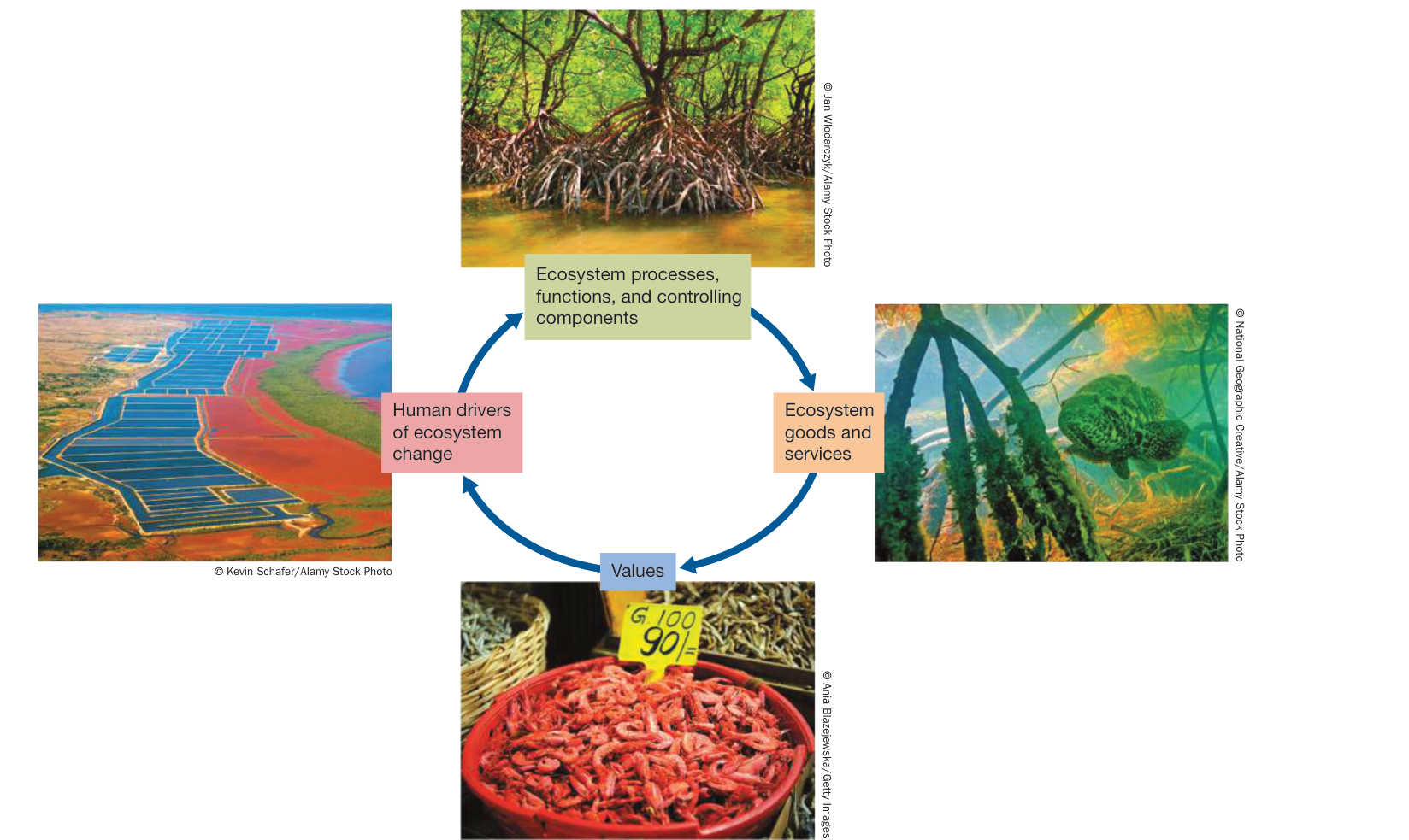
Figure 56.18 Key Steps to Ecosystem Service Valuation Placing a value on ecosystem services, such as this mangrove ecosystem used for shrimp farming, involves determining (1) the human drivers of ecosystem change, (2) the ecosystem processes or functions affected by those changes, (3) how those processes or functions affect the delivery of goods and services of an ecosystem, and (4) the willingness of people to pay for those goods and services.
Recap and Assess
Ecosystems provide benefits to humans in the form of goods and services. Ecologists recognize different categories of services depending on their role in the ecosystem. Ecosystem service valuation, important to establish sustainable practices, involves determining the market value or the willingness of people to pay for the services.
- Suppose you want to maximize the coastal protection service of mangroves with shrimp aquaculture farming (which requires removing the mangrove trees to create ponds). What sustainable solution might you devise to maximize the value of this ecosystem?

Activity 56.3 Concept Matching: Ecosystems
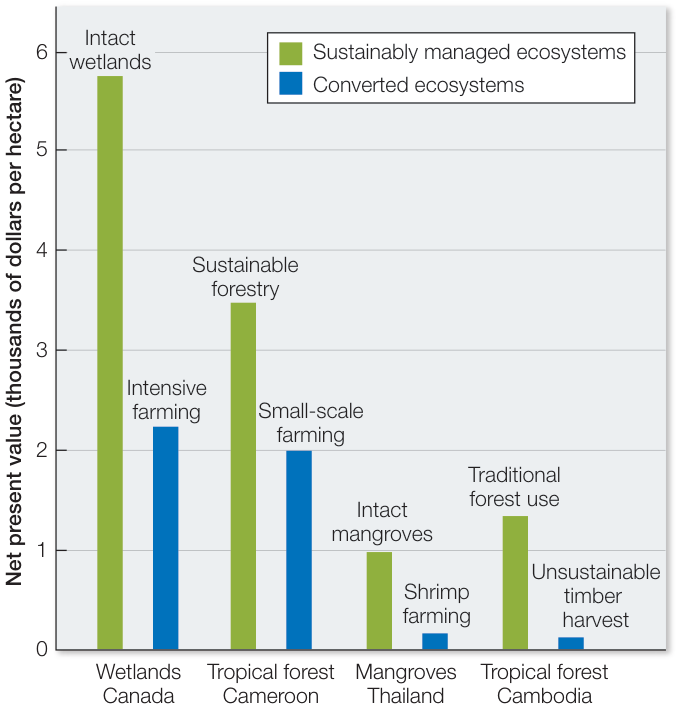
Figure 56.19 The Economic Value of Sustainability Managed Ecosystems Many types of ecosystems are able to provide more goods and services, and thus have a higher value, when they are sustainably managed than when they are completely converted to human use. (From Millennium Ecosystem Assessment, 2005. Ecosystems and Human Well-being: Synthesis. Island Press: Washington, DC. © 2005 World Resources Institute.)
Investigating Life
QA How will food webs respond to the multiple effects of ocean acidification and warming in marine ecosystems?
Much of the ocean acidification research to date has focused on the responses of single species to increasing CO2 and warming. While we know that ocean acidification and warming can have negative effects on calcifying organisms, potentially affecting already compromised coral-reef ecosystems, we know much less about the potentially counteracting effects of elevated CO2 on primary producers and their consumers. Is it possible that organisms, placed within the context of their food webs, gain some resilience from the effects of climate change? The study of a Swedish estuary showed that the response of this ecosystem to ocean acidification and warming is modulated by complex food web interactions. The implications of this study may be wide-ranging if changes in food webs decrease the ability of ecosystems to respond to climate change. Will the loss of top consumers make ecosystems less resilient to climate change? This is a question that needs to be considered as both food webs and global climate change.
Future directions
While the Swedish estuary experiment shows that a consumer can affect an ecosystem’s response to climate change, climate change can also affect a consumer’s role in an ecosystem. A good example is the recent dramatic shift in polar bear and orca observations in the Canadian Arctic. Sea ice in the Arctic is melting at unprecedented rates as the result of global warming. Polar bears need this sea ice to stalk their prey, mainly seals, and have been driven to inland hunting grounds with the loss of ice. Orcas, by contrast, are unable to hunt their preferred prey—other species of whales—in ice-covered waters. As ice continues to melt, orcas have been spotted in areas of the Arctic where they have never been seen before. Some people have suggested that this shift from seal predation to whale predation could have important ecosystem-level effects as the food webs shift in response to the decline of sea ice.

Visual Summary

© Cameron Davidson/Getty Images
You should be able to relate each summary to the adjacent figures. If you go to this visual summary in Achieve, you can follow links to figures, animations, activities, and simulations that will help you consolidate the material.
Ecosystem Science Considers
- ■ An ecosystem includes all the organisms in a given area and their physical and chemical environment.
- ■ Energy flowing through ecosystems originates with sunlight and inorganic and organic compounds. It involves the processes of photosynthesis, chemosynthesis, and secondary production.
- ■ Energy is lost from ecosystems as metabolic heat.
- ■ Nutrients originate in soil, water, and the atmosphere and cycle through ecosystems via the processes of production and decomposition.
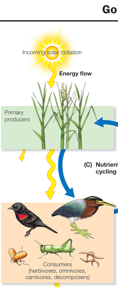
Figure 56.1
Questions
- How are ecosystems the same and different from communities?
- What are the sources of energy that flow through ecosystems?
- How do nutrients cycle through ecosystems?
Energy and Nutrients in
- ■ Net primary production (NPP) is the amount of carbon remaining in plants after respiration, and varies with latitude and ecosystem type.
- ■ Terrestrial NPP is highest in the tropics where temperatures are high year-round and rainfall is abundant.
- ■ Oceanic NPP varies little with latitude but peaks at mid-latitudes and in coastal zones and areas of upwelling where the main primary producers—phytoplankton and algae—have access to light and nutrients.
- ■ In aquatic systems, nutrient runoff from agriculture and wastewater can cause eutrophication, resulting in algal blooms and low oxygen conditions (hypoxia) for aquatic life.
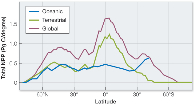
Figure 56.2
Questions
- How does net primary production differ from gross primary production?
- What are the latitudinal patterns and processes important to net primary production in terrestrial versus oceanic ecosystems?
- What are the causes and consequences of eutrophication in aquatic systems?
Food Webs Transfer Energy
- ■ Once energy captured by primary producers is fixed as NPP, consumption by heterotrophs transfers a fraction of that energy to higher trophic levels, creating net secondary production.
- ■ Organisms differ in their production efficiency—the percentage of energy stored in assimilated food that is used to produce new biomass.
- ■ The amount of energy transferred within food webs depends on trophic efficiency—the amount of energy used at one trophic level divided by the amount used at the trophic level below it.
- ■ The flow of energy in food webs is influenced by the relative contribution of bottom-up (NPP passing up the food web) and top-down (consumers regulating NPP) forces, the number of trophic levels, and the presence of omnivory.
- ■ Most food webs have just three or four trophic levels because of energy limitations at higher trophic levels, the effects of disturbance, or the evolutionary constraints on top predators.
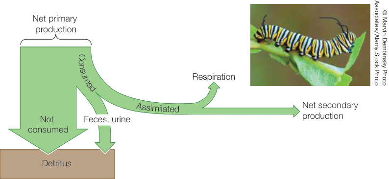
Figure 56.8
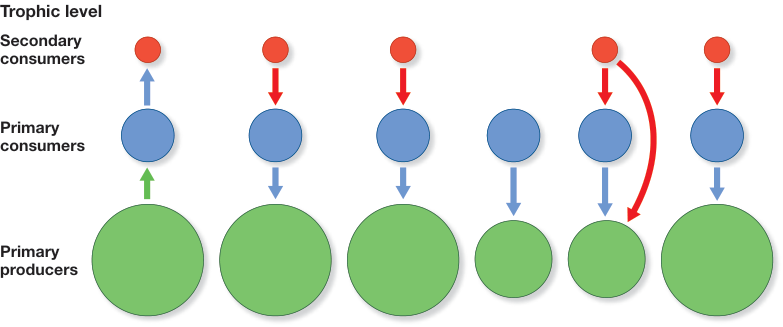
Figure 56.10
Questions
- How and why do production efficiencies differ between ectotherms and endotherms?
- How is energy flow in food webs influenced by the relative contributions of bottom-up and top-down forces, number of trophic levels, and the presence of omnivory?
- What are three factors hypothesized to be important in determining food chain length?
- Nutrients move through the biotic parts of ecosystems via production and decomposition.
- At a global scale, nutrients move through geological, atmospheric, and biological pools, making up biogeochemical cycles.
- Water cycles rapidly through the globe as part of the hydrologic cycle, transporting nutrients and serving as an essential requirement for organisms.
- Carbon moves through biological systems and returns to the atmosphere through respiration.
- Burning of fossil fuels increases the carbon dioxide and sulfur in the atmosphere, causing global warming and acidic conditions in oceans and lakes.
- The nitrogen cycle is dominated by biotic transformations controlled by bacteria, whereas the phosphorus and sulfur cycles are dominated by geochemical processes.
Questions
- What is the role of decomposition and mineralization in nutrient cycling?
- Describe Earth’s carbon cycle and how fossil-fuel burning is raising global temperatures.
- Describe the role of microbes versus that of geological processes in global nitrogen, phosphorus, and sulfur cycles.
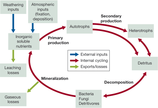
Figure 56.11
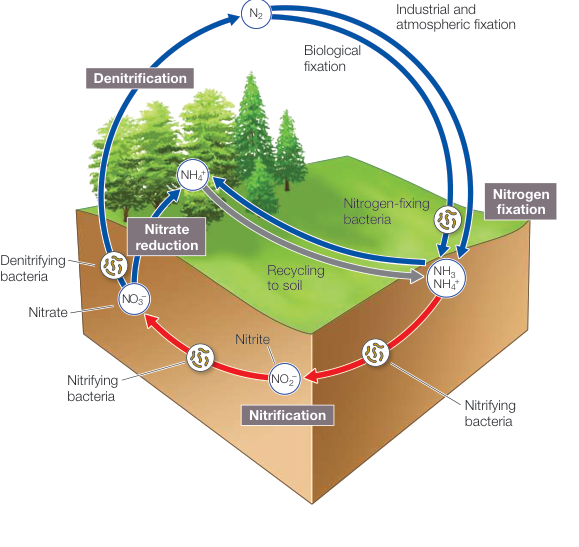
Figure 56.16
Ecosystems Provide Important
- Ecosystem services benefit humans and can be categorized as providing provisioning, regulating, supporting, or cultural services.
- Most ecosystem services are either irreplaceable or prohibitively expensive to replace.
- Ecosystem values are measures of how important ecosystem services are to people—that is, what they are worth.
- Ecosystem services can be valued by determining the market value or the willingness of people to pay for the services.
Questions
- Describe the four categories of ecosystem services.
- How can humans promote sustainability and reduce ecosystem service trade-offs?
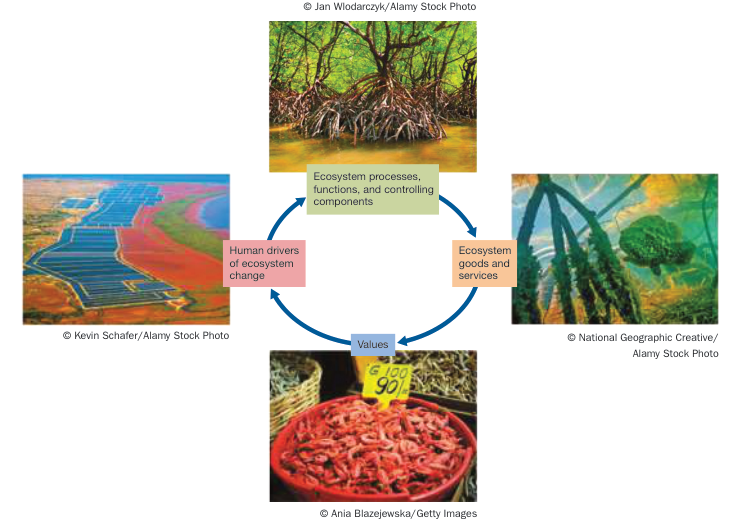
Figure 56.18