Chapter 3Proteins and NMR Structural Biology
As mentioned in the previous chapter, one-dimensional NMR techniques, which yield extremely useful information in small molecules, are of limited applicability to the complex, highly overlapped spectra of biological macromolecules. To effectively use the information available from NMR spectroscopy of biological macromolecules, we introduced multidimensional NMR spectroscopy. It combines data from several kinds of spectra to establish the mappings for resonance assignments. In general, there are two types of multidimensional spectra, homonuclear spectra, in which each axis represents the same type of atom (usually protons), and heteronuclear spectra, in which each axis represents a different type of atom. In this lecture, we briefly introduce several essential multidimensional NMR experiments and techniques.
COSY
Homonuclear correlation spectroscopy (COSY) is two-dimensional, and shows the frequencies for a single isotope (usually protons) along both axes of the spectrum. As shown in figure 3.1, the COSY spectrum consists of a series of peaks on the diagonal, and the peaks that appear off of the diagonal are called cross-peaks. These cross-peaks are symmetrical (above and below the diagonal) and indicate which protons are spin-spin coupled with each other. Therefore, by matching the center of a cross-peak with the center of each of two corresponding diagonal peaks, one can determine which atoms are connected to one another by chemical bonds. The peaks on the diagonal and the matched cross-peaks are coupled to each other.
The three-dimensional () experiment is designed to accurately determine three-bond J-coupling constants (also called scalar couplings). While the NOE provides information on the distance between two nuclei, this J-coupling constant is dependent on the dihedral angle in the structure. In particular, this coupling constant provides information about the dihedral angles subtended by the coupled atoms. For example, we can derive the dihedral angle by mapping J-coupling constants in the Karplus curve as shown in figure 3.2.
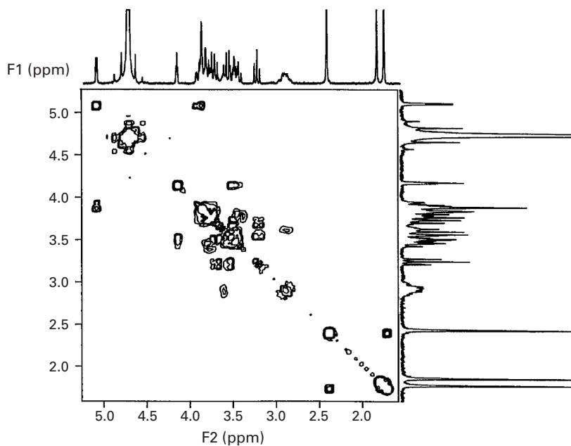
Figure 3.1 COSY spectrum of proton-proton scalar couplings.
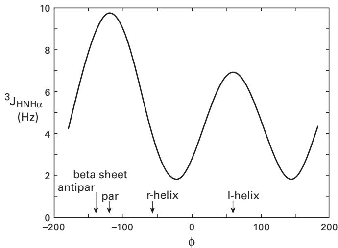
Figure 3.2 The Karplus relationship between the three-bond coupling constant and the torsional angle . The Karplus curve is calculated as , where , , and are empirically derived parameters. Credit: http://www.cryst.bbk.ac.uk/PPS.
HSQC
Heteronuclear Single Quantum Correlation (HSQC) is one of the most important two-dimensional NMR experiments. It correlates the nitrogen atom of an NH moiety with the directly attached proton, and each signal in an HSQC spectrum represents a proton that is bound to a nitrogen atom. Since every residue except proline has (ideally) a unique pair on the protein backbone and ideally has distinct frequency signals, the HSQC spectrum can serve as the identification (“hash code”) of each residue, and reference interaction for all other spectra. The HSQC spectrum also contains signals from the NH groups of the side-chains, such as Asn and Gln and the aromatic protons of Trp and His. Unlike homonuclear spectra, the HSQC spectrum has no diagonal because different nuclei are observed during the relaxation periods and (figure 3.3).
TOCSY
3D Total Correlation Spectroscopy (TOCSY) is a three-dimensional (3D) heteronuclear NMR experiment. In contrast to the HSQC, TOCSY experiments record the side-chain protons as the third axis in the spectrum. Figure 3.4 shows a TOCSY spectrum by fixing the atoms from 3D data, in which the peaks are from side-chain protons and , and the strips group atoms by the spin system. In this spectrum, the -axis is the shift; the -axis shows the and the side-chain shifts, and the -axis (projected out) gives the shift. Given the fact that the chemical shifts of protons for different amino acids are characteristically different, we can regard these strips (number and position of peaks) as the “fingerprints” of the protons to identify probable amino acid types.
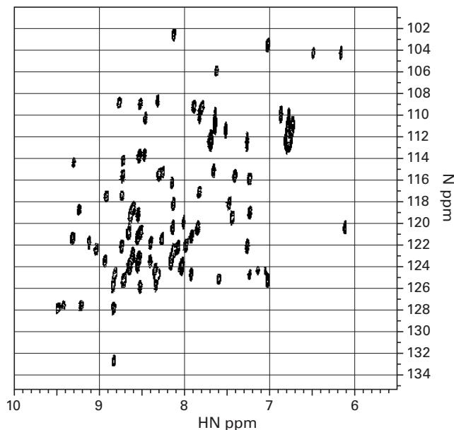
Figure 3.3 The NMR spectrum of HSQC.
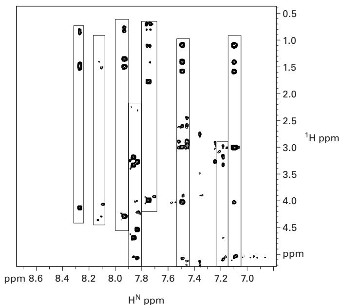
Figure 3.4 The NMR spectrum of TOCSY. Each strip indicates atoms grouped by the spin system.
Having constrained the amino acid type for each peak in HSQC from TOCSY experiments, in order to obtain actual assignments, we still need to establish the sequential connectivities between spin systems. Generally, we combine information from different NMR experiments by cross-referencing peaks to reveal the sequential connectivities, for example, HN(CO)CA and HNCA. These correlate the , , and nuclei in a residue, and in the previous residue in the protein. Note that prolines will not generate peaks in any spectrum that involves the backbone amide, for example, HSQC, NH(CO)CA, HNCA, TOCSY.
NOESY
The Nuclear Overhauser Effect (NOE) is caused by dipolar coupling between nuclei, that is, the local field at one nucleus is affected by the presence of another nucleus. The intensity of the interactions is (ideally) a function of the distance between the nuclei according to the following equation
where is the intensity that is measured, is a scaling constant, and is the distance between nuclei. In other words, NOE provides a link between an experimentally measurable quantity, , and internuclear distance. NOEs are measured with NOE spectroscopy (NOESY) experiments. For example, 3D NOESY, a 3D heteronuclear NMR experiment, measures the through-space NOE between an amide proton and a neighboring , when they are within a distance less than 6 Å. In a NOESY experiment, the height and volume of the peak gives the intensity, and is related to the distance between the two atoms: Bigger peaks indicate close distance, and weak peaks indicate that the atoms are further apart and/or moving.
RDC
Residual dipolar couplings (RDCs) [2], which were first proposed in the 1980s, have emerged as an important tool in NMR to study macromolecular structure and function in a solution environment. In typical NMR experiments, the protein is in water (or water and deuterium) and it tumbles isotropically. However, if the molecules in solution exhibit a partial alignment, for example, after adding an alignment medium to the solution, this leads to incomplete averaging of spatially anisotropic dipolar couplings, and RDCs between two spins will be measured.
RDCs are complementary to NOEs; they provide global orientational information as opposed to local distance information (NOEs). RDCs also contain distance information as well as measuring the angles that are formed by a vector connecting the two atoms within a tensor axis system. In addition, both NOEs and RDCs can be used as restraints by algorithms for protein structure determination.
RDCs are defined in terms of a coordinate system called the principal order frame (POF). The general formula to extract bond orientations using RDCs for two spins and , as described in figure 3.5, is as follows:
where is the residual dipolar coupling, measured in units of Hertz, is Planck’s constant, is the gyromagnetic ratio, is the interspin distance, is the angle between the interspin vector and the external magnetic field, and and are the spins. Then, we can simplify the equation as (see chapter 5, or [3] for details)
where is a physical constant, is the orientation of the bond vector in the POF, and is a symmetric and traceless matrix, which contains 5 degrees of freedom, called the alignment tensor (or Saupe matrix). In practice, the dipolar coupling is measured directly, and the matrix and the vector are initially unknown. However, given a putative model, we can solve for (via singular value decomposition) and back-compute RDCs. The difference between the computed and observed RDCs () can be used to refine the model. denotes the ensemble average. When and are covalently bonded, we typically know this distance from empirical crystal structures and replace by a scalar distance .
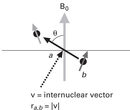
Figure 3.5 Extracting bond orientations using RDCs: Spins and are in the magnetic field ; and indicate the orientation and the distance between the spins and , respectively.
Summary
There are many NMR experiments. Let us summarize the ones we have discussed so far.
Multidimensional NMR Experiments
Sequential connectivity via and other backbone chemical shifts
Sequential connectivity of HSQC peaks
Amino acid types
J-coupling ( angles)
NOESY distance ()
Data Type and Information Content
Chemical shifts Resonance frequencies (chemical shifts)
Scalar couplings Dihedral angular constraints (local)
NOEs Distance constraints
Residual dipolar couplings Global orientation constraints
More Applications of NMR Solvent accessibility, dynamics, protein folding assays, protein interaction assay, SAR by NMR, and others.
References
- [1] John Cavanagh, et al.: Protein NMR Spectroscopy : Principles and Practice 2nd ed. New York: Academic Press, 2007.
- [2] R. S. Lipsitz and N. Tjandra. Residual dipolar couplings in NMR structure analysis. Annual Review Biophysics Biomolecular Structure 2004. 33: 387–413.
- [3] S. Grzesiek. EMBO short course on RDCs. Accessed: 2006. http://www.embl-heidelberg.de/nmr/sattler/embo/handouts/grzesiek\_RDC.pdf
- [4] Kurt Wuthrich. NMR of Proteins and Nucleic Acids. New York: John Wiley & Sons, 1996.
- [5] P. J. Hore. Nuclear Magnetic Resonance. New York: Oxford University Press, 1995.
- [6] Horst Friebolin. Basic One-and Two-Dimensional NMR Spectroscopy. Weinheim: VCH Pub., 1998.