Chapter 22ROCK and FRODA for Protein Flexibility
This chapter describes two examples of using the algorithmic approach FIRST to explore protein flexibility: ROCK [1, 2] and FRODA [3]. FIRST is introduced in chapter 21.
The ROCK Algorithm
Terminology
Ring A closed loop of bonds in which any two atoms are connected by two distinct paths.
Interlocked rings Two rings that share common bond(s).
Ring cluster A collection of rings that are interlocked with one another.
Side branches All atoms that do not belong to any ring cluster.
Figure 22.1 shows examples of ring, interlocked ring, ring cluster, and side branch.
Overview
Rigidity Optimized Conformational Kinetics (ROCK) is an algorithm that generates conformations for a protein that satisfy the flexibility constraints. ROCK explores flexible regions identified by FIRST by a random-walk sampling of the rotatable bonds.
The following shows the steps of the ROCK algorithm:
- Get the flexibility information from FIRST (chapter 21).
- Generate conformations for ring clusters. Reject unclosed conformations.
- Attach and perturb side branches. Reject conformations with steric clash or bad bond length/angles.
- Reject conformations with bad stereochemistry (analogous to the Ramachandran plot for proteins).
- Reject conformations with missing hydrophobic interactions.
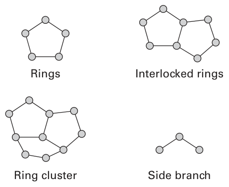
Figure 22.1 Examples of ring, interlocked ring, ring cluster, and side branch.
Conformation Sampling in Single-Ring Closure
Although it is easy to generate conformations for side branches, it is not trivial to generate conformations for ring clusters, since the dihedral angles in a ring are all correlated.
An -fold ring closes if the following equations are satisfied:
where is the distance vector, is the rotational matrix along the bond angle, and is the rotational matrix along the dihedral angle.
The total DOFs of an -fold ring are . If dihedral angles in an -fold ring are fixed, the remaining six dihedral angles can be obtained by solving the ring closure equations. Conformational sampling in an -fold ring is performed by altering dihedral angles randomly and then computing the remaining six unknown dihedral angles by solving the ring closure equations.
Conformation Sampling in Multiple-Ring Closure
First, a fictitious closure potential is defined by
To close all rings, we need to minimize , the total fictitious potential of all rings in the ring cluster. In a closed ring cluster, the total fictitious potential is minimized to zero.
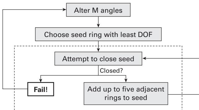
Figure 22.2The iterative approach for minimizing the total fictitious ring closure potential.
Suppose that we have a set of dihedral angles in an -atom ring cluster, then computing the minimum value of the total fictitious potential takes time, which is not feasible for large . An improved approach is to iteratively close rings, that is, to close one ring in the ring cluster at each iteration. Let denote the total number of rings. Since the average number of variables per ring is , the total computational cost is , which is when . In practice, however, it is impossible to close all the rings in an interlocked ring cluster iteratively, since closing some rings unavoidably opens other rings. ROCK applies an iterative scheme to solve the ring closure equations of all rings in a ring cluster, as shown in figure 22.2.
Conformation Sampling in Side Branches
After new conformations of the ring clusters have been generated, side branches are set with correct bond lengths and angles. The atomic positions in side branches are first randomly perturbed, and then relaxed such that (1) bond lengths and angles of side branch atoms are maintained; (2) there are no van der Waals overlaps between side branches themselves, nor between side branches and ring clusters; and (3) chirality at side branches is maintained. A nonlinear optimization toolbox (DONNLP2) is used to find the optimal solutions of side branches while satisfying these constraints.
Hydrophobic Interactions and Ramachandran Checks
Once each new conformation is generated, the distances between pairs of carbon atoms need to be checked to determine whether they are in the hydrophobic interaction list. The new conformation is accepted if the distances are within the allowed hydrophobic interaction distance; otherwise it is rejected.
The dihedral angles are also checked against the Ramachndran plot. Conformations with bad stereochemistry are rejected.
Application of ROCK in Flexible Docking
The following steps show how to apply ROCK in protein-ligand flexible docking:
- Analyze rigidity of protein and ligand by using FIRST.
- Apply ROCK to generate conformations for protein and ligand.
- Apply SLIDE to dock all possible pairs of conformations.
SLIDE is a modeling tool for protein-ligand interactions based on steric complementarity, hydrophobic, and hydrogen-bonding interactions.
FRODA
Overview
Framework rigidity optimized dynamic algorithm (FRODA) is designed for exploring the internal mobility of proteins. In FRODA, the rigid regions of the protein are first identified by using FIRST, and replaced by ghost templates that guide the movements of atoms. The conformational space is explored using random moves. The covalent, hydrophobic, and hydrogen bond constraints, and the avoidance of van der Waals overlaps are all considered.
The FRODA Algorithm
In FRODA, a ghost template represents a rigid body that consists of a set of mutually rigid atoms. Atoms are bound to the vertices of the ghost templates. The following iterative process is used to enforce the bond length/angle constraints: The ghost templates are fit to the atom positions by using a least-squares approach, and then atoms are fit to the vertices to which they are bound. During geometric simulation of the protein motions, we vary some dihedral angles while keeping the bond length and angle constraints unchanged. For intuition, imagine there are only two ghost templates. The preceding iterative process is quite similar to the expectation/maximization approach in linear regression, and will typically converge to a new conformer. For example, in an E/M linear regression problem, we are given a set of points in an Euclidean space, and try to find two optimal lines that best fit these points. A difference between the linear regression and the iterative process here may be that, not only the lines (corresponding to the ghost templates) but also the points (corresponding to atoms) are allowed to move, which in fact speeds up the convergence. Figure 22.3 (plate 23) shows a simulation example from an ethane molecule’s motion.
The steric clash problem is handled by adding a small bias to the atomic motion during the fitting process between atoms and templates, as shown in figure 22.4 (plate 24). A similar method is also applied to ensure hydrophobic relationships. The Ramachandran plot is used to check and reject conformers with bad ( , ) dihedral angles.
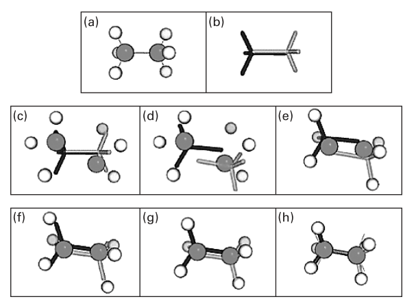
Figure 22.3 (plate 23) The motion of an ethane molecule as determined by geometric simulation: (a) Initial atomic positions; (b) ghost templates; (c) random atomic displacement; (d) fitting of ghost templates to atoms; (e) refitting of atoms to ghost templates; (f) and (g) further iterations of (d) and (e); (h) until a new conformer is found [3].
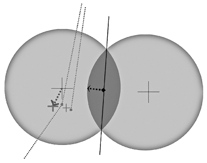
Figure 22.4 (plate 24) The method to handle steric overlap. When atoms come into contact, the overlap influences the movement of the atoms during the relaxation. The atom on the left is tethered to sites (blue dots) in two ghost templates (shown as blue dotted lines). The center of the atom, shown as a large black cross, would move to the small light blue cross in order to match the midpoint of its two associated ghost template sites. However, the steric overlap (black dashed arrows) causes it to move further away from the touching atom, so that its new position is at the larger blue cross, and the resultant motion is shown by the dashed red arrow [3].
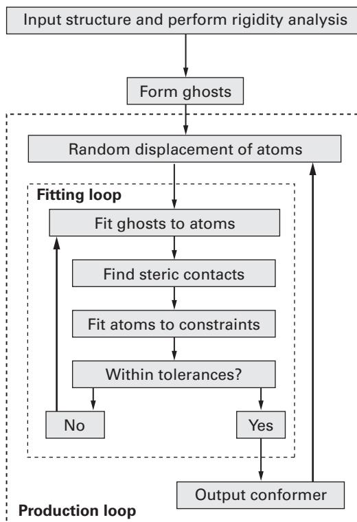
Figure 22.5 The program flow of the FRODA algorithm. An initial rigidity analysis leads to the creation of the ghost templates. Each iteration of the FRODA loop involves an initial random displacement of the atoms followed by multiple iterations of the fitting loop, in which the geometric and steric constraints are enforced [3].
Figure 22.5 shows the flow of the FRODA algorithm, and figure 22.6 (plate 25) illustrates the exploration of the conformation space.
Comparisons Between ROCK and FRODA
FRODA is much faster (about 100 to 1,000 times) than ROCK, since ROCK spends a lot of time in rejecting possible conformers, while FRODA does not solve expensive closure equations or perform nonlinear optimization.
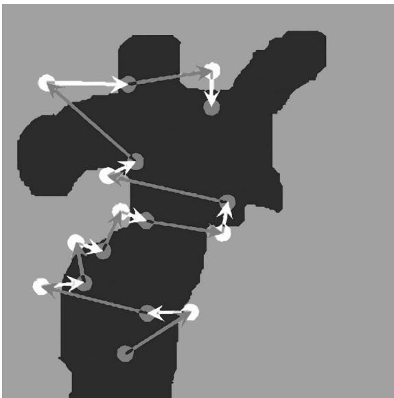
Figure 22.6 (plate 25) Exploration of the conformation space. Here we show a sketch of a two-dimensional slice through the 3N-dimensional phase space of the protein, divided into allowed (blue) and forbidden (red) zones. Successive random moves (green arrows) followed by enforcement of the constraints (yellow arrows) produces a set of conformers (green circles) that explore the allowed region [3].
References
- [1] M. Lei, M. I. Zavodszky, L. A. Kuhn, and M. F. Thorpe. Sampling protein conformations and pathways. Journal of Computational Chemistry 25(2004):1133–1148.
- [2] M. I. Zavodszky, M. Lei, M. F. Thorpe, A. R. Day, and L. A. Kuhn. Modeling correlated main-chain motions in proteins for flexible molecular recognition. Proteins: Structure, Function, and Genetics 44(2004):150–165.
- [3] S. Wells, S. Menor, B. Hespenheide, and M. F. Thorpe. Constrained geometric simulation of diffusive motion in proteins. Physical Biology 2, (2005):S127–S136.