Families, alignments, and profiles
Give a structure predictor one sequence and it has little to go on. Give it the sequence's relatives, stacked in an alignment, and it can see which residues each position tolerates across the family. That is why predictors from the early secondary-structure networks to AlphaFold take an alignment, or a profile built from one, rather than the bare sequence. Here you'll read an alignment column by column and turn it into numbers.
Families record which changes a structure tolerates
Positions in the hydrophobic core, in active sites, on the surface, and on the interface between protein domains each have their own rules, stemming from the fact that similar mutations at different positions would lead to different effects for the entire protein: some would be easily accepted, while others will not. For this reason, a uniform mutation matrix, the same at every position along the sequence, does not provide a good description of the evolutionary process under strong pressure of preserving the structure and function of a protein. A set of position-specific mutation rules can be derived from the analysis of a multiple alignment of a homologous family and subsequently used to align new sequences in this family. This idea, in various forms and under different names (profile, position-specific mutation matrix, or hidden Markov models of protein families), allowed sequence analysis methods to break through the twilight zone and reliably recognize distant homologues even when their sequence identity was much below 25% and comparison of single sequences appeared random.
About 67 out of 100 residues can be exchanged in a protein without changing structure. On the other hand, exchanges of very few residues often destabilize a protein structure. The explanation for this ostensible contradiction is simple: evolution has realized the unlikely by exploring all neutral mutations that do not prevent structure formation. Thus, the residue exchange patterns extracted from an aligned protein family are highly indicative of specific structural details. This also implies that a profile of a few consecutive residues taken from alignments implicitly contains nonlocal information. The source of this information is that evolutionary selection acts on a 3D object (the protein) rather than on an abstracted 1D construct (the sequence).
Reading a multiple sequence alignment
A multiple sequence alignment (MSA) stacks related sequences so that each column holds residues
descended from the same ancestral position. Rows are sequences and columns are positions, with a gap
character (- or .) where a sequence has no residue at that position. Finding the optimal alignment of many
sequences at once is NP-hard, so programs build them heuristically: progressively along a guide tree (a
rough phylogenetic tree built from pairwise similarities, aligning the closest pairs first), or by aligning
every sequence to a statistical model of the family.
Here are the first rows of Pfam's curated "seed" alignment for the ubiquitin family (Pfam is a public database of protein families; more on it at the end of this lesson). The family includes ubiquitin itself and many proteins that carry a ubiquitin-like domain inside a longer chain:
import gzip
import urllib.request
import numpy as np
from primer import CACHE, display_html

def pfam(accession, kind="seed"):
    """A Pfam family alignment (Stockholm format) as {name: aligned sequence}, downloaded once."""
    path = CACHE / f"{accession.lower()}-{kind}.sto.gz"
    if not path.exists():
        url = f"https://www.ebi.ac.uk/interpro/api/entry/pfam/{accession}/?annotation=alignment:{kind}"
        request = urllib.request.Request(url, headers={"User-Agent": "study-bioprimer"})
        path.write_bytes(urllib.request.urlopen(request, timeout=300).read())
    rows = {}
    for line in gzip.open(path, "rt"):
        if line.strip() and not line.startswith(("#", "//")):
            name, seq = line.split()
            rows[name] = rows.get(name, "") + seq.upper().replace(".", "-")
    return rows

seed = pfam("PF00240")
names = list(seed)
msa = np.array([list(seed[n]) for n in names])
print(f"{len(names)} sequences, {msa.shape[1]} columns")

CLASS = {**dict.fromkeys("AVLIMFWY", "#eda100"), **dict.fromkeys("STNQ", "#1baf7a"),
         **dict.fromkeys("KRH", "#2a78d6"), **dict.fromkeys("DE", "#e34948"), **dict.fromkeys("GPC", "#6250d6")}
def colored(row):
    return "".join(f'<span style="color:{CLASS.get(c, "#aaa")}">{c}</span>' for c in row)
display_html("<pre style='font-size:12px;line-height:1.25'>" +
             "\n".join(f"{n[:20]:20s} {colored(seed[n][:60])}" for n in names[:14]) + "</pre>")
59 sequences, 89 columns
OASL_HUMAN/436-507   VFVKN--PDGG-----SYAY-AINPNSFILGLKQQIEDQQ-G---LPKKQQ-QLEFQGQV
RS30_HUMAN/3-72      LFVRA----QE-----LHTF-EVTGQETVAQIKAHVASLE-G---IAPEDQ-VVLLAGAP
Q18231_CAEEL/3-69    IFLLG--LDNT-----THTL-DVDASTTLSAIKGVIG---------AGEEF-SISYGSKV
ISG15_HUMAN/84-155   ILVRN--NKGR-----SSTY-EVRLTQTVAHLKQQVSGLE-G---VQDDLF-WLTFEGKP
ISG15_BOVIN/81-152   ILVRN--DKGR-----SSPY-EVQLKQTVAELKQQVCQKE-R---VQADQF-WLSFEGRP
ISG15_MOUSE/82-153   ILVRN--ERGH-----SNIY-EVFLTQTVDTLKKKVSQRE-Q---VHEDQF-WLSFEGRP
YKA4_CAEEL/343-415   ILIKLKFMNDT-------------EKNTYASLEDTVAKFKVDHFTNLANQVIRLIYQGQL
R7SL1_ARATH/3-74     VYIDT--ETGS-----SFSI-TIDFGETVLEIKEKIEKSQ-G---IPVSKQ-ILYLDGKA
Q9ZQZ4_ARATH/3-74    MTVEN--ESGS-----TFSI-DIGLQDTVLTFKRKIEMTQ-R---IPVSRQ-TIFFQGKL
Q9VEC8_DROME/3-75    ITIKV--LKGK-----DCTI-EVAPTSTILEVKHQIEAEL-Q---ISATNQ-KLLLLGRP
UBL4A_MOUSE/3-74     LTVKA--LQGR-----ECSL-QVAEDELVSTLKHLVSDKL-N---VPVRQQ-RLLFKGKA
PRKN_MOUSE/3-74      VFVRF--NSSY-----GFPV-EVDSDTSILQLKEVVAKRQ-G---VPADQL-RVIFAGKE
Q9VXF9_DROME/3-75    ITVTT--SDDK-----VFCL-DVAQDLELENLKALCAMEI-G---AEVSQI-AVIFNGRE
SUMO_CAEEL/15-88     IKIKVVGQDSN-----EVHF-RVKYGTSMAKLKKSYADRT-G---VAVNSL-RFLFDGRR
Multiple sequence alignments represent the main source of evolutionary information available. The relation between equivalent positions of homologous proteins compiles the result of the changes allowed by the evolution of the corresponding proteins at different positions.
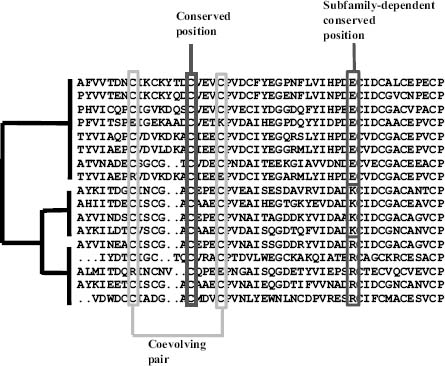
Features of a multiple sequence alignment and its implicit phylogeny. Conserved positions are invariant throughout all the sequences. In family-dependent conserved positions, a different amino acid type is conserved within each subfamily. For coevolving pairs of positions, changes in one position are correlated with changes in the other.
Conserved positions are invariable positions, interpreted as important residues for the structure or function of the protein since apparently changes were disallowed during evolution. Conserved positions usually are located in structural cores (structurally important positions) and active or binding sites (positions directly involved in protein function). Although locating conserved positions could look trivial at first sight, different approaches produce different results depending, for example, on the treatment of conservative changes. Modern methods take into account the phylogeny of the sequences in the alignment, so as to avoid artifacts due to an uneven distribution of sequences in the alignment (highly similar sequences resulting in most of the positions being conserved).
Family-dependent conserved positions are a more subtle kind of conservation. These positions are typically conserved in the subfamilies that form well-defined branches of the phylogenetic tree and differ in the chemical type of the amino acids that characterize each subfamily. Family-dependent conserved positions are most likely related with the specific features of each subfamily, which in most cases turn out to be differential binding to other proteins and substrates (the molecules an enzyme acts on).
The third kind of position in the figure, coevolving pairs, is the subject of lesson 5.4.
A profile is a distribution per column
A profile replaces each column with a probability distribution over the 20 amino acids. That's the "1D" representation of a family that structure-prediction networks take as input, one 20-vector per residue. Computing it is counting, with one decision to state up front: what to do about gaps.
You can ignore gaps, dividing each residue count by the number of sequences that have a residue in that column. The distribution then describes what the position is when it exists, and you report the gap fraction separately. Or you can count the gap as a 21st symbol and divide by the number of sequences, so columns where many sequences have gaps get flatter residue frequencies.
On a small alignment you can do it by hand:
toy = ["PQITLWQRPLV",
       "PQVTLWKRPLV",
       "PQITLWQRPIV",
       "PEISLWRRPLV",
       "PQ-TLWQ-PLV"]
AA = "ACDEFGHIKLMNPQRSTVWY"

for j in range(len(toy[0])):
    column = [s[j] for s in toy]
    residues = [c for c in column if c != "-"]
    freqs = {a: residues.count(a) / len(residues) for a in sorted(set(residues))}
    gaps = column.count("-") / len(column)
    print(f"column {j + 1:2d}: {column}  ->  {freqs}  gaps {gaps:.0%}")
column  1: ['P', 'P', 'P', 'P', 'P']  ->  {'P': 1.0}  gaps 0%
column  2: ['Q', 'Q', 'Q', 'E', 'Q']  ->  {'E': 0.2, 'Q': 0.8}  gaps 0%
column  3: ['I', 'V', 'I', 'I', '-']  ->  {'I': 0.75, 'V': 0.25}  gaps 20%
column  4: ['T', 'T', 'T', 'S', 'T']  ->  {'S': 0.2, 'T': 0.8}  gaps 0%
column  5: ['L', 'L', 'L', 'L', 'L']  ->  {'L': 1.0}  gaps 0%
column  6: ['W', 'W', 'W', 'W', 'W']  ->  {'W': 1.0}  gaps 0%
column  7: ['Q', 'K', 'Q', 'R', 'Q']  ->  {'K': 0.2, 'Q': 0.6, 'R': 0.2}  gaps 0%
column  8: ['R', 'R', 'R', 'R', '-']  ->  {'R': 1.0}  gaps 20%
column  9: ['P', 'P', 'P', 'P', 'P']  ->  {'P': 1.0}  gaps 0%
column 10: ['L', 'L', 'I', 'L', 'L']  ->  {'I': 0.2, 'L': 0.8}  gaps 0%
column 11: ['V', 'V', 'V', 'V', 'V']  ->  {'V': 1.0}  gaps 0%
Column 7 is a distribution, Q 60%, K 20%, and R 20%, rather than a single letter. A consensus sequence would write "Q" and throw the rest away. How peaked a column is can be measured by its Shannon entropy, . A column with one residue has ; a column with all 20 equally likely has bits. The information content is high where the family is constrained, and a sequence logo draws it: each column is a stack of letters whose total height is the information and whose letter heights are the frequencies.
Code
from primer import display_widget

keep = [j for j in range(msa.shape[1]) if (msa[:, j] == "-").mean() < 0.5]   # the family model's positions
alphabet = AA + "-"
counts = [[int((msa[:, j] == a).sum()) for a in alphabet] for j in keep]
ubq = "MQIFVKTLTGKTITLEVEPSDTIENVKAKIQDKEGIPPDQQRLIFAGKQLEDGRTLSDYNIQKESTLHLVLRLRGG"
labels = [f"{ubq[k + 2]}{k + 3}" for k in range(len(keep))]   # these 72 columns are ubiquitin residues 3-74
display_widget(
    "sequence-logo",
    "A sequence logo of the ubiquitin family's 72 core columns, labeled with the human ubiquitin residue at "
    "each position. Scroll sideways. Switch between counting gaps and ignoring them, and add pseudocounts to "
    "see how a few pretend observations flatten columns from a small alignment. Hover a column for its numbers.",
    counts=counts, labels=labels,
)
A sequence logo of the ubiquitin family's 72 core columns, labeled with the human ubiquitin residue at each position. Scroll sideways. Switch between counting gaps and ignoring them, and add pseudocounts to see how a few pretend observations flatten columns from a small alignment. Hover a column for its numbers.
Two refinements turn raw frequencies into a profile you can score with:
The first is sequence weighting. Databases are lumpy: twenty near-identical sequences from close relatives would outvote one distant homolog twenty to one, though together they carry about one sequence's worth of information. A common fix weights each sequence by one over the number of sequences at least 80% identical to it. The sum of the weights, the effective number of sequences, measures how much an alignment knows.
The second is pseudocounts. With 60 sequences, a residue never seen in a column gets frequency zero, and a score built on would forbid it forever. Adding a few pretend observations, spread in proportion to background frequencies or to what BLOSUM says can substitute for what was seen, keeps every residue possible but unlikely.
A position-specific scoring matrix (PSSM) then scores residue at position with : lesson 5.2's log-odds, but with a different target distribution at every position. Scoring a new sequence against a PSSM means summing these along an alignment to the profile. The same dynamic programming works with a profile column in place of a residue.
Conservation maps onto structure
The profile was computed from sequences alone. Compare its information content with the structure of human ubiquitin, using relative solvent accessibility from lesson 2.4:
from Bio.PDB.SASA import ShrakeRupley
from primer import structure

MAX_ASA = {"ALA": 129, "ARG": 274, "ASN": 195, "ASP": 193, "CYS": 167, "GLN": 225, "GLU": 223,
           "GLY": 104, "HIS": 224, "ILE": 197, "LEU": 201, "LYS": 236, "MET": 224, "PHE": 240,
           "PRO": 159, "SER": 155, "THR": 172, "TRP": 285, "TYR": 263, "VAL": 174}

def information(column, pseudo=0.5):
    residues = [c for c in column if c in AA]                     # gaps ignored
    p = (np.array([residues.count(a) for a in AA]) + pseudo) / (len(residues) + 20 * pseudo)
    return np.log2(20) + (p * np.log2(p)).sum()

info = np.array([information(list(msa[:, j])) for j in keep])
chain = structure("1UBQ")[0]["A"]
ShrakeRupley().compute(chain, level="R")
residues = [r for r in chain if r.id[0] == " "][2:74]               # residues 3-74
rsa = np.array([r.sasa / MAX_ASA[r.get_resname()] for r in residues])

print(f"mean information: buried positions {info[rsa < 0.2].mean():.2f} bits, "
      f"exposed {info[rsa >= 0.2].mean():.2f} bits")
rank = lambda x: np.argsort(np.argsort(x))
print(f"rank correlation of information with exposure: {np.corrcoef(rank(info), rank(rsa))[0, 1]:.2f}")
print("most conserved positions:")
for k in np.argsort(-info)[:8]:
    r = residues[k]
    print(f"  {r.get_resname()} {r.id[1]:2d}: {info[k]:.2f} bits, {rsa[k]:.0%} exposed, column {''.join(msa[:, keep[k]])[:24]}…")
mean information: buried positions 1.32 bits, exposed 0.97 bits
rank correlation of information with exposure: -0.52
most conserved positions:
  GLY 47: 2.99 bits, 64% exposed, column GGSGGGGGGGGGGGGGGGGGGGGG…
  LYS 27: 2.60 bits, 1% exposed, column KKKKKKEKKKKKKKKMMMKKKKKK…
  LEU 50: 2.35 bits, 2% exposed, column LLLLMMLLLLLLLIIIILLLLLLL…
  LEU 43: 2.10 bits, 0% exposed, column LVILLLLLILLVVFFFFFILLLLL…
  ASP 52: 2.00 bits, 20% exposed, column DDEDDDDDDNDNDDDAPADDDDDN…
  VAL  5: 1.86 bits, 0% exposed, column VVLVVVIIVIVVVILLLLVVIIVV…
  LEU 67: 1.84 bits, 0% exposed, column LLLVVVVLLLLVIIIIIILVIVLF…
  ILE  3: 1.81 bits, 0% exposed, column VLIIIIIVMILVIIIIIILVLILI…
Buried positions average 1.32 bits against 0.97 for exposed ones (rank correlation with exposure −0.52), and each of the most conserved positions has a structural job. Most are core hydrophobics, which change only among Leu, Ile, Val, and Met. Gly47 sits in a tight turn that only glycine's backbone fits. Lys27 is almost completely buried, unusual for a lysine, because its charge is paired with the partly buried Asp52, which is also conserved: a buried salt bridge (lesson 1.4).
Ubiquitin with its most conserved positions from the family profile: core residues in amber, Gly47 in violet, and the buried Lys27–Asp52 salt bridge with its 2.9 Å distance. Every one of these was found from sequence variation alone.
Open 1UBQ in Mol*Profile hidden Markov models and Pfam
Hidden Markov models are perhaps the most successful approach for modeling protein domain families. For an alignment of a family of homologous protein domain sequences, HMMs capture the distribution of residues at each conserved position as well as the likelihood of deletions and insertions at or between the conserved positions. HMMs best model whole superfamilies, while multiple models should be built for subclusters within each superfamily. The full diversity of a superfamily cannot be adequately captured in a single model, as superfamilies frequently contain sequences with low pairwise identity that cannot be successfully aligned.
A profile HMM is a profile with explicit gap states. Each family position has a match state that emits residues from that column's distribution, an insert state for extra residues between positions, and a delete state for skipping the position, with transition probabilities between them. Aligning a sequence to the model is the Viterbi algorithm, dynamic programming again, and the result is a log-odds score against a background model. HMMER is the standard implementation.
Pfam is a database of more than 20,000 such families. Each has a hand-curated seed alignment, like the one above, from which a model is built. The model is then searched against all of UniProt to produce the full alignment: the ubiquitin family's has about 90,000 sequences. The pipelines that feed AlphaFold build their alignments the same way. Tools such as jackhmmer and HHblits search huge sequence databases iteratively: find relatives, build a profile from them, search again with the profile, and repeat.
Check yourself
In an alignment of 40 sequences, column 17 contains 30 leucines and 10 gaps; column 18 contains 10 each of Leu, Ile, Val, and Met. Which column is more conserved, and how does your answer depend on the gap policy?
Reasoning
Ignoring gaps, column 17 is a single residue (entropy 0, maximal information), but only 75% of sequences have a residue there, so it may be a position some relatives lost, often in a loop. Counting gaps as a symbol, its distribution is 75% L and 25% gap, entropy about 0.81 bits, still well conserved. Column 18 has four residues equally (entropy 2 bits) under either policy, but they are all large hydrophobics. A plain entropy calls it moderately variable, yet it is constrained to "buried hydrophobic", which a BLOSUM-aware measure or a pseudocount scheme based on substitution groups would recognize. Report the gap fraction alongside any conservation score.
An alignment contains 50 sequences of mouse, rat, and human versions of one protein and 3 distant homologs from bacteria. Every column looks conserved. Why is that misleading, and what would you do?
Reasoning
The 50 mammalian sequences are nearly identical because they diverged recently, not because every position is constrained. They carry about one sequence's worth of information, but unweighted counting gives them 50 votes. Weight the sequences (one over the number of neighbors above 80% identity) or cluster them first. The effective number of sequences here is perhaps 4, which is not enough to say much about conservation. You'd want to gather more diverse homologs.
A residue on the surface of an enzyme is invariant across 500 diverse homologs. What does that suggest, and how could you check it with a structure?
Reasoning
Surface positions normally vary freely, so an invariant surface residue is under a constraint beyond folding: most likely function, as part of an active site, a binding site, or an interface with a partner. Map it onto the structure and see whether it clusters with other conserved surface residues into a patch or a pocket, near a bound ligand or cofactor if one is present. Conserved and exposed residues that cluster together are the classic signature of a functional site.