Helices, sheets, turns, and loops
The allowed regions of the Ramachandran plot are not equally used: most residues in a folded protein sit in one of two repeating patterns, the α-helix and the β-strand. Secondary structure was the first thing structure prediction learned to predict, and it is still the first thing to look at in a model.
The secondary structure of a protein can be thought of as the local conformation of the polypeptide chain, independent of the rest of the protein. Two types of secondary structure have emerged as the dominant local conformations of polypeptide chains: the alpha (α) helix and beta (β) sheets. These structures were predicted by Linus Pauling, Robert Corey, and H.R. Branson, based on the known physical limitations of polypeptide chains, before any protein structure had been determined experimentally. Helices and sheets contain φ and ψ angles that fall within the two largest regions of allowed conformation, and they exhibit a high degree of regularity: the particular φ and ψ angle combinations are approximately repeated for the duration of the secondary structure.
Although helices and sheets satisfy the peptide bond constraints, this is not the only factor that explains their ubiquity. Both of these structural elements are stabilized by hydrogen bond interactions between the backbone atoms of the participating residues. Helices and sheets are the only regular secondary structural elements present in proteins. However, irregular secondary structural elements are also observed in proteins and are vital to both structure and function.
α-helices
A helix is created by a curving of the polypeptide backbone such that a regular coil shape is produced. Because the polypeptide backbone can be coiled in two directions (left or right), helices exhibit handedness. Almost all helices observed in proteins are right-handed, as steric restrictions limit the ability of left-handed helices to form. Among the right-handed helices, the α-helix is by far the most prevalent.
An α-helix is distinguished by having a period of 3.6 residues per turn of the backbone coil. The structure of this helix is stabilized by hydrogen bonding interactions between the carbonyl oxygen of each residue and the amide proton of the residue four positions ahead in the helix.Chemists often call a hydrogen bonded to N or O a "proton", since it is the part that can leave as H⁺. The amide proton is the H on the backbone N. Consequently, all possible backbone hydrogen bonds are satisfied within the α-helix, with the exception of a few at each end of the helix, where a partner is not available.
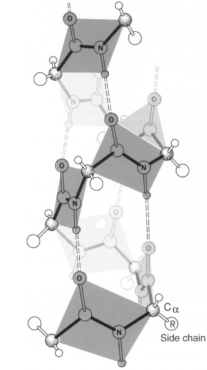
An α-helix. Dashed lines are the hydrogen bonds from each carbonyl oxygen to the amide hydrogen four residues ahead. The backbone curves to the right, so the helix is right-handed.
The α helix is a right-handed coil that turns in the same clockwise direction as a standard wood screw. The R groups extend outward from the peptide backbone of the helix.
Every residue in an α-helix has the same (φ, ψ), about (−57°, −47°) in the ideal helix and (−63°, −43°) on average in real ones. Give every residue the same pair of angles and the chain has to become a regular helix, because each residue is related to the next by the same rotation and translation (a screw motion). The two angles set everything else. For the α-helix that is 3.6 residues per turn, 100° of rotation and 1.5 Å of rise per residue, and a pitch (rise per turn) of 5.4 Å. Try it here:
A chain built from one (φ, ψ) pair, repeated. The readout measures residues per turn, rise, and handedness from the built coordinates; dashed lines are backbone hydrogen bonds (N–O under 3.5 Å), colored by how far apart in sequence the partners are. Pick a preset, or press Fold from extended to sweep from a stretched chain to the target. The small map shows the pair on the Ramachandran plot. Yellow spheres are Cβ atoms: they point outward and back toward the N-terminus.
Handedness comes from φ and ψ. The left-handed α preset, (+57°, +47°), is the mirror image: the same 3.6 residues per turn, turning the other way. For L-amino acids it sits in the cramped αL corner of the map, which is why long left-handed helices don't occur and right-handed ones are everywhere.
The 3₁₀ helix at (−49°, −26°) is tighter, with 3.0 residues per turn and a 2.0 Å rise, and its hydrogen bonds jump three residues (i → i+3) instead of four. Its name records this: 3 residues per turn, 10 atoms in the ring closed by each hydrogen bond. (In the same notation the α-helix is a 3.6₁₃ helix.) 3₁₀ segments are short, often a single turn at the end of an α-helix. The π-helix at (−57°, −70°) is wider, about 4.3 residues per turn, with i → i+5 bonds; it shows up as a one-turn bulge inside an α-helix where one extra residue has been inserted.
The β and PPII presets have no internal hydrogen bonds at all. An extended chain has to find its partners elsewhere.
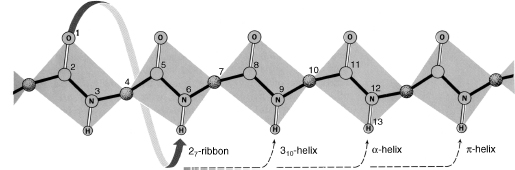
Hydrogen-bond partners for each helix type, drawn on a stretched-out backbone: i+3 for the 3₁₀ helix, i+4 for the α-helix, i+5 for the π-helix. (The 2₇ ribbon is shown for completeness; it is not a regular structure.)
All the peptide groups in a helix point the same way along its axis, and each is a small electric dipole, so a helix carries a partial positive charge at its N-terminus and a partial negative charge at its C-terminus. The first four N–H groups and the last four C=O groups have no partners inside the helix. Side chains that can satisfy them, such as Ser, Thr, Asp, and Asn at the N-terminus ("N-caps") and Gly at the C-terminus, are common right at helix ends, and phosphate groups often bind at helix N-termini.
β-strands and sheets
Unlike helices, β-sheets are formed by hydrogen bonds between adjacent polypeptide chains rather than within a single chain. Sections of the polypeptide chain participating in the sheet are known as β-strands. β-strands represent an extended conformation of the polypeptide chain. This arrangement produces a sheet that is pleated, with the residue side chains alternating positions on opposite sides of the sheet.
Two configurations of β-sheet are possible: parallel and antiparallel. In parallel sheets, the strands are arranged in the same direction with respect to their amino terminal (N) and carboxy terminal (C) ends. In antiparallel sheets, the strands alternate their amino and carboxy terminal ends, such that a given strand interacts with strands in the opposite orientation. β-sheets can also form in a mixed configuration, with both parallel and antiparallel sections. Almost all β-sheets exhibit some degree of twist when viewed along the strands. This twist is generally right-handed.
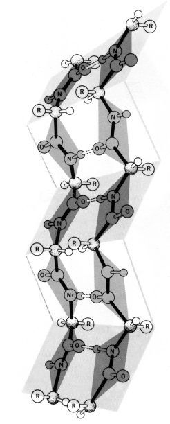
An antiparallel β-sheet. Dashed hydrogen bonds join the carbonyl oxygen of a residue on one strand to the amide hydrogen of a residue on the next. The sheet is pleated, and side chains alternate above and below it.
The hydrogen bonds tell the two kinds of sheet apart. In an antiparallel pair, residue i on one strand and its partner j on the other bond to each other twice (N–H of i to C=O of j and back), and the next bonded pair is two residues along. In a parallel pair, residue i bonds to j−1 with its N–H and to j+1 with its C=O, so the bonds slant across the gap. Ubiquitin has both kinds. The cell below finds every backbone hydrogen bond with the electrostatic energy that DSSP uses (described further down), then prints the ladders between its strands:
import numpy as np
from primer import fetch, structure, sequence

chain = structure("1UBQ")[0]["A"]
res = [r for r in chain if r.id[0] == " "]
num = [r.id[1] for r in res]
N, CA, C, O = (np.array([r[a].coord for r in res]) for a in ("N", "CA", "C", "O"))

# DSSP puts each amide H 1.0 Å from N, in the direction of the previous residue's O=C bond, reversed.
H = N.copy()
H[1:] = N[1:] + (C[:-1] - O[:-1]) / np.linalg.norm(C[:-1] - O[:-1], axis=1, keepdims=True)

def hbond_energy(i, j):
    """Electrostatic energy (kcal/mol) of C=O of residue i accepting from N–H of residue j."""
    d = lambda a, b: np.linalg.norm(a - b)
    return 0.084 * 332 * (1 / d(O[i], N[j]) + 1 / d(C[i], H[j]) - 1 / d(O[i], H[j]) - 1 / d(C[i], N[j]))

n = len(res)
hb = {(i, j) for i in range(n) for j in range(1, n) if abs(i - j) > 1 and hbond_energy(i, j) < -0.5}
print(len(hb), "backbone hydrogen bonds (O of i ← N–H of j);",
      sum(j - i == 4 for i, j in hb), "of them are i → i+4")

def ladder(a, b):
    """Hydrogen bonds between residue ranges a and b, as (acceptor O, donor N–H) residue numbers."""
    pairs = sorted((num[i], num[j]) for i, j in hb if (num[i] in a and num[j] in b) or (num[i] in b and num[j] in a))
    return " ".join(f"{o}←{h}" for o, h in pairs)

print("strand 1–7 with 10–17 (a hairpin):  ", ladder(range(1, 8), range(10, 18)))
print("strand 1–7 with 64–72:              ", ladder(range(1, 8), range(64, 73)))
54 backbone hydrogen bonds (O of i ← N–H of j); 12 of them are i → i+4
strand 1–7 with 10–17 (a hairpin):   1←17 3←15 5←13 7←10 11←7 13←5 15←3
strand 1–7 with 64–72:               2←64 4←67 6←69 65←4 67←6
In the hairpin, the partners in every bond add up to 18: 1←17, 3←15 and 15←3, 5←13 and 13←5. (Residue 1's reverse bond is missing because the N-terminal nitrogen has no modeled hydrogen.) Residues 1 and 17, 3 and 15, and 5 and 13 face each other directly, bonded both ways, and the strands run in opposite directions. Between strands 1–7 and 64–72 the bonds slant. Residue 4's C=O takes the N–H of 67 while its own N–H gives to the C=O of 65 (4←67 and 65←4), so residue 4 sits across from 66 and bonds to the residues on either side of it. Residue 6 does the same around 68. That is a parallel pair.
Turns and loops
In order for β-strands to interact with each other and form a sheet, the backbone must form a turn. The simplest and tightest turn is the β-hairpin turn (also called type I and type II turns, depending on the conformation of the backbone). Other stereochemically allowed turns include the mirror images of the type I and type II turns (denoted type I′ and type II′) as well as type III and type VI turns. All are observed in naturally occurring proteins; the type I turn appears to be most commonly used.
An important variant of the classical β-sheet structure is the β-bulge, most often observed in antiparallel β-sheets: a hydrogen bond between two residues on one β-strand with one residue on the adjacent strand. This structure can alter the direction of the polypeptide chain and augment the right-handed twist of the sheet.
α-helices and β-sheets account for the majority of secondary structure seen in proteins. However, these regular structures are interspersed with regions of irregular structure that are referred to as loop or coil. Loop regions are usually present at the surface of the protein. These regions are often simply transitions between regular structures, but they can also possess structural significance and can be the location of the functional portion, or active site, of the protein.
β-hairpin turns involve the minimum number of residues (4–5); transitions involving more residues (6–16) are often referred to as omega (Ω) loops because they resemble the shape of the capital Greek letter omega. These loops can involve complex interactions that include the side chains, in addition to the polypeptide backbone.
Although loop regions are irregular, these structures are generally as well ordered as the regular secondary structures. However, experimental determination of protein structures has shown that some loop regions are disordered and thus do not achieve a stable structure. This type of loop region is referred to as random coil.
A β-turn spans four residues, i to i+3, and reverses the chain's direction. It is closed by one hydrogen bond from the C=O of residue i to the N–H of residue i+3, the same i → i+3 bond as one turn of 3₁₀ helix. The two middle residues set the type: type I has (φ, ψ) near (−60°, −30°) then (−90°, 0°), and type II has (−60°, 120°) then (80°, 0°). That second residue's positive φ is why type II turns usually have a glycine at position i+2. Ubiquitin's hairpin turn is type I: Leu 8 sits at (−73°, −7°) and Thr 9 at (−101°, 15°), and the C=O of Thr 7 bonds to the N–H of Gly 10 (the 7←10 bond in the output above). Gly 10 itself has φ = +77°. The "ordered" claim also has a structural test: a loop that holds the same conformation in every copy of the protein in a crystal, and in every model of an NMR ensemble (an NMR structure is deposited as a bundle of models that all fit the data; unit 6), is ordered. Lesson 3.5 takes up loops and whole proteins that are not.
Secondary structure as a string
We may view the peptide chain as a sequence loop(u loop)*, where the term u is either an α-helix or a β-strand and the term "loop" is possibly empty. This structure is referred to as the secondary structure. As defined, the secondary structure should be viewed as possessing some mechanical flexibility. If the bonds in the α and β components impart some local rigidity, the loop components are eminently flexible. This enables the various terms of the secondary structure to come in mutual proximity and to realize additional bonds. The resulting structure is called tertiary.
So secondary structure can be written as one label per residue, a string the same length as the sequence. Programs that assign it from coordinates mostly work from the hydrogen bonds:
DSSP, by Kabsch and Sander, performs its sheet and helix assignments based on the backbone–backbone hydrogen bonds. DSSP defines a hydrogen bond when the bond energy is below −0.5 kcal/mol, from a Coulomb approximation of the hydrogen bond energy. An α-helix assignment (DSSP state "H") starts when two consecutive residues have i → i+4 hydrogen bonds. This definition is also used for 310-helices (state "G", with i → i+3 hydrogen bonds) and for π-helices (state "I", with i → i+5 hydrogen bonds). Single helix hydrogen bonds are assigned as turns (state "T").
β-sheet residues (state "E") are defined as either having two hydrogen bonds in the sheet, or being surrounded by two hydrogen bonds in the sheet. Isolated residues fulfilling this hydrogen bond criterion are labeled as β-bridge (state "B"). The remaining two DSSP states "S" and blank indicate a bend in the chain and the unassigned/other state, respectively.
DSSP continues to be the most widely used method, and most prediction methods are based on DSSP assignments. Typically, the eight DSSP states are converted into three classes using the following convention: [GHI] → H, [EB] → E, [TS and blank] → C. 310-, α-, and π-helices are grouped into one helix class; extended β-sheets and β-bridges are grouped into one sheet class; and the remaining states (turn, bend, and "not assigned") are grouped into one coil class. An alternative conversion yields a seemingly higher level of prediction accuracy: [H] → H, [E] → E, [GIBTS and blank] → C.
The cell above used that energy test. Here is ubiquitin's sequence with its three-state labels from the file's HELIX and SHEET records, scored against a made-up prediction that moves a few boundaries and misses the short helix at 56–59, the typical mistakes of real predictors:
seq = sequence(chain)
true = ["C"] * n
for line in fetch("1UBQ").read_text().splitlines():
    if line.startswith(("HELIX", "SHEET")):
        start, end = (int(line[21:25]), int(line[33:37])) if line.startswith("HELIX") else (int(line[22:26]), int(line[33:37]))
        for k in range(start, end + 1):
            true[num.index(k)] = "H" if line.startswith("HELIX") else "E"
true = "".join(true)
predicted = "CEEEEEECCCCEEEEECCCCCCHHHHHHHHHHHHCCCCCCEEEECCCEECCCCCCCCCCCCCEEEEEEECCCCCCC"

for k in range(0, n, 25):
    print(f"{k + 1:>3} {seq[k:k + 25]}\n    {true[k:k + 25]}  file\n    {predicted[k:k + 25]}  predicted\n")
q3 = sum(a == b for a, b in zip(true, predicted)) / n
print(f"Q3 = {q3:.0%} of residues labeled correctly")
  1 MQIFVKTLTGKTITLEVEPSDTIEN
    EEEEEEECCEEEEEEEECCCCCHHH  file
    CEEEEEECCCCEEEEECCCCCCHHH  predicted

 26 VKAKIQDKEGIPPDQQRLIFAGKQL
    HHHHHHHHHCCCCCEEEEEECCEEE  file
    HHHHHHHHHCCCCCCEEEECCCEEC  predicted

 51 EDGRTLSDYNIQKESTLHLVLRLRG
    CCCCCHHHHCCCCEEEEEEEEECCC  file
    CCCCCCCCCCCCEEEEEEECCCCCC  predicted

 76 G
    C  file
    C  predicted

Q3 = 80% of residues labeled correctly
Q3, the fraction of residues with the right label, is the standard score for secondary-structure prediction; the best current methods reach about 85% on proteins they have not seen. Even a perfect label string is far from a structure, though. It says which residues are helical, not where the helix sits, which strands pair, or whether a pair is parallel. Two proteins with identical label strings can have different folds.
Contact maps
A label string can't tell you which strand pairs with which. A contact map can. Take one representative atom per residue (usually Cβ, or Cα for glycine), compute all pairwise distances to get an n × n matrix, and mark the pairs closer than a cutoff, conventionally 8 Å. The matrix is symmetric, and because it is built from distances it does not change when the molecule is rotated or translated. That invariance is why contact maps (and distance maps) are a natural target for prediction networks, including the first versions of AlphaFold.
Each kind of secondary structure leaves a signature:
- a helix is a thick band along the diagonal, because residue i touches i+3 and i+4;
- an antiparallel pair of strands is a band perpendicular to the diagonal, because as one strand goes up in sequence its partner goes down;
- a parallel pair is a band parallel to the diagonal, off to the side.
Ubiquitin's contact map, beside its structure. Strips along the edges mark the helices (orange) and strands (blue). Hover over any cell to see that residue pair in 3D. Find the hairpin (1–7 with 10–17) just off the diagonal at the top left, the parallel pair 1–7 with 64–72 in the top-right corner, and the helix 23–34 on the diagonal. Switch to distances to see the whole matrix, and move the cutoff to see how the counts change.
Ubiquitin colored by the HELIX and SHEET records in its file. The five strands form one mixed sheet: the first two are antiparallel (the hairpin), and the first and the strand at 64–72 run parallel.
Open 1UBQ in Mol*Check yourself
A 20-residue α-helix has how many i → i+4 backbone hydrogen bonds, and how many backbone N–H and C=O groups go unpaired inside it? How long is it, end to end?
Reasoning
The C=O of residue i bonds to the N–H of i+4 for i = 1 to 16, so there are 16 bonds. The first four N–H groups (residues 1–4) and the last four C=O groups (residues 17–20) have no partner, which is why capping residues and solvent matter at helix ends. Length: 20 residues × 1.5 Å = 30 Å, about the thickness of the hydrophobic core of a lipid bilayer. That is why membrane-spanning helices are about 20 residues long (lesson 3.5).
In a contact map you see a band of contacts running from (10, 40) to (16, 34). Is this a helix, a parallel sheet, or an antiparallel sheet, and which residues pair?
Reasoning
As the first index goes up (10 → 16) the second goes down (40 → 34): the band runs perpendicular to the diagonal, so it is an antiparallel pair of strands. Residue 10 pairs with 40, 11 with 39, and so on to 16 with 34. The constant sum (50) is the antiparallel signature. A parallel pair would keep a constant difference instead.
A secondary-structure predictor scores Q3 = 80% on a protein. Give two ways the 20% of mistakes could be nearly harmless, and one way they could be badly misleading for building a 3D model.
Reasoning
Harmless: the errors could all be at segment ends, where a helix is called one residue too long or too short; or a short 3₁₀ helix is called coil, which barely changes the fold. Misleading: the same 20% could be one entire strand missed, or a strand called a helix. That changes how many strands are in the sheet and what pairs with what, and a 3D model built on it would have the wrong topology, meaning the wrong order and pairing of strands and helices. Q3 counts residues, not segments, so it can't tell these cases apart.