The Ramachandran plot
The last lesson reduced a backbone to two angles per residue, so every residue is a point on a 360° × 360° square. Most of that square is forbidden: at most (φ, ψ) pairs, two atoms would overlap. You'll compute the forbidden part from nothing but atom sizes, then drop real proteins on top and see how well hard spheres predict them. The same plot is one of the first checks run on any structure, experimental or predicted.
Steric hindrance shrinks the space
Rotational freedom about the φ (Cα–N) and ψ (Cα–C) angles is limited by steric hindrance between the side chains of the residues and the peptide backbone. A Ramachandran plot (a plot of φ versus ψ angles) maps the entire conformational space of a polypeptide and illuminates the allowed and disallowed conformations. These plots were developed by G.N. Ramachandran in the 1960s based on studies of sterically allowed φ and ψ angle combinations.
Some exceptions to these conformational limitations can be attributed to glycine and proline. The side chain of glycine (a single hydrogen atom) is very small. There is markedly reduced steric hindrance about the φ and ψ angles of this residue, thus expanding the possible conformational space. Conversely, the cyclic bond present in proline residues reduces the conformational freedom beyond the limitations observed with other amino acids.
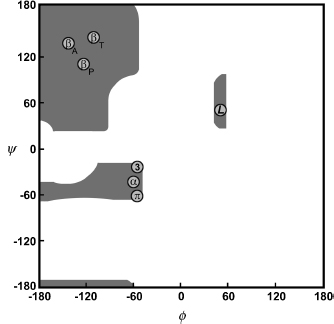
A schematic Ramachandran plot. Grey regions are allowed conformations of the backbone. Circles mark the angle pairs of the repetitive secondary structures: βA, antiparallel β-sheet; βP, parallel β-sheet; βT, twisted β-sheet; α, right-handed α-helix; L, left-handed helix; 3, 310 helix; π, π-helix.
Computing the map from hard spheres
Ramachandran's method is simple enough to run in a browser. Treat atoms as hard spheres. For each pair of atoms, a table gives the closest they can come: 3.2 Å for two carbons, 2.7 Å for nitrogen and oxygen, 2.0 Å for two hydrogens, and so on. A slightly smaller "outer limit" for each pair allows for atoms that can squeeze a little. Then, for every (φ, ψ) on a grid:
- Build three residues with ideal bond lengths and angles: the Cα, C, and O of residue i−1, all of residue i, and the N, H, and Cα of residue i+1.
- Measure every atom pair whose distance depends on φ or ψ. Pairs fixed by the bonds are skipped.
- Shade the cell if no pair is closer than its outer limit.
The figure below does this live, for alanine (whose side chain is a single methyl group) or glycine. Ubiquitin's and protein kinase A's residues are drawn on top of it.
Code
import math
from Bio.PDB import PPBuilder
from primer import structure, display_widget

def phi_psi(pdb_id, chain):
    """(φ, ψ, residue name, residue number) for every residue that has both angles."""
    out = []
    for peptide in PPBuilder().build_peptides(structure(pdb_id)[0][chain]):
        for res, (phi, psi) in zip(peptide, peptide.get_phi_psi_list()):
            if phi is not None and psi is not None:
                out.append([round(math.degrees(phi)), round(math.degrees(psi)), res.get_resname(), res.id[1]])
    return out

points = phi_psi("1UBQ", "A") + phi_psi("1ATP", "E")
display_widget(
    "ramachandran-explorer",
    "The hard-sphere map with the residues of ubiquitin (1UBQ) and protein kinase A (1ATP) on top. Drag the "
    "red cursor: the 3D view shows the three-residue model at that (φ, ψ), with overlapping atoms joined in red "
    "and tight contacts in amber. Switch to glycine, or change the N–Cα–C bond angle τ.",
    points=points,
)
The hard-sphere map with the residues of ubiquitin (1UBQ) and protein kinase A (1ATP) on top. Drag the red cursor: the 3D view shows the three-residue model at that (φ, ψ), with overlapping atoms joined in red and tight contacts in amber. Switch to glycine, or change the N–Cα–C bond angle τ.
Three things to try in it:
- Put the cursor at φ = ψ = 0. The carbonyl oxygen of residue i−1 lands on the amide hydrogen of residue i+1, 0.3 Å apart. Most of the plot fails like this, with one specific pair of atoms colliding.
- Switch to glycine. Its Hα is much smaller than alanine's Cβ, so whole regions open on the right half of the plot, and the allowed area becomes nearly symmetric under (φ, ψ) → (−φ, −ψ). Glycine has no chiral center (lesson 1.6), so its mirror-image conformations are equally possible.
- Move τ, the N–Cα–C bond angle, from 110° to 115°. Real τ values spread over several degrees (ubiquitin's are 110° ± 4°), and the αR region grows noticeably as τ opens up. At 115°, about 90% of the real residues fall inside the hard-sphere map. The ones that don't sit mostly at the edges of the helix and bridge regions, where real atoms squeeze slightly closer than hard spheres allow.
The regions and their names
Four regions hold almost every non-glycine residue in a real protein. Each one corresponds to a repeating structure that lesson 3.3 builds:
| Region | Typical (φ, ψ) | What sits there |
|---|---|---|
| αR, right-handed helix | (−63°, −43°) | α-helices and 3₁₀ helices, plus isolated helical residues in loops |
| β, extended | (−120°, +130°) | β-strands; antiparallel strands a little more extended than parallel |
| PPII, polyproline II | (−75°, +145°) | a left-handed extended helix with three residues per turn; common in loops and unfolded chains |
| αL, left-handed helix | (+57°, +47°) | mostly glycine, sometimes asparagine or aspartate, usually single residues in turns |
The bottom-left and right-hand parts of the plot are empty for every residue except glycine. The β and PPII regions sit next to each other and real residues spread between them.
The same picture drawn from data, with glycine and proline in their own panels:
import numpy as np
import matplotlib.pyplot as plt

everything = points + phi_psi("7RSA", "A") + phi_psi("1A6M", "A")
phi, psi, name = (np.array([p[i] for p in everything]) for i in range(3))

fig, axes = plt.subplots(1, 3, figsize=(10, 3.6), sharey=True)
groups = [("other residues", (name != "GLY") & (name != "PRO"), "#333333"),
          ("glycine", name == "GLY", "#6250d6"), ("proline", name == "PRO", "#eb6834")]
for ax, (title, mask, color) in zip(axes, groups):
    ax.scatter(phi[mask], psi[mask], s=7, color=color, alpha=0.7)
    ax.set(xlim=(-180, 180), ylim=(-180, 180), xticks=[-180, -90, 0, 90, 180], yticks=[-180, -90, 0, 90, 180],
           title=f"{title} ({mask.sum()})", xlabel="φ (degrees)")
    ax.axhline(0, color="#dddddd", lw=0.8, zorder=0)
    ax.axvline(0, color="#dddddd", lw=0.8, zorder=0)
axes[0].set_ylabel("ψ (degrees)")
plt.tight_layout()
plt.show()

pro_phi = phi[name == "PRO"]
print(f"proline φ: mean {pro_phi.mean():.0f}°, range {pro_phi.min():.0f}° to {pro_phi.max():.0f}°")
print(f"glycine with φ > 0: {(phi[name == 'GLY'] > 0).mean():.0%};"
      f" other residues with φ > 0: {(phi[(name != 'GLY') & (name != 'PRO')] > 0).mean():.0%}")
proline φ: mean -61°, range -84° to -24°
glycine with φ > 0: 55%; other residues with φ > 0: 2%
Across ubiquitin, protein kinase A, ribonuclease A, and myoglobin, ordinary residues pack into the αR and β regions. Over half the glycines sit at φ > 0, against 2% of everything else. Proline stays in a narrow band around φ = −65°: its side chain loops back and bonds to its own backbone nitrogen, closing a five-membered ring around the N–Cα bond, so φ can't swing far. Proline's nitrogen also has no hydrogen to donate to a hydrogen bond, one reason it disrupts helices and sheets.
The plot as a quality check
The next passage borrows a few terms from unit 6. In brief: an X-ray experiment produces a 3D electron density map, a blurry cloud showing where the electrons are. A person or program refines an atomic model to fit it. Resolution is roughly the finest detail the data can show, so a smaller number is sharper. R-free scores how well the model predicts a slice of the data held back from fitting, much like a validation-set error. NMR is a second experimental method that measures proteins in solution.
For proteins, the best known, and most powerful, check of stereochemical quality is the Ramachandran plot. In the φ–ψ scatterplot, the points tend to be excluded from certain "disallowed" regions and have a tendency to cluster in certain favorable regions.
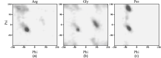
Observed φ–ψ distributions in a representative sample of protein structures for (a) arginine, a fairly standard residue, (b) glycine, and (c) proline. Darker regions are more densely populated.
The favorable regions on the plot correspond to the regular secondary structures: right-handed helices, extended conformation (as found in β-strands), and left-handed helices. Even residues in loops tend to lie within these favored regions.
One caveat concerns proteins containing D-amino acids rather than the more common L-amino acids. These residues have the opposite chirality so their φ–ψ values will be negative with respect to their L-amino cousins. The Ramachandran plot for D-amino acids is the same as for L-amino acids, but with every point reflected through the origin. Thus, proteins such as gramicidin A, which have many D-amino acids, give Ramachandran plots that look particularly troubling, but which may be perfectly correct.
The tightness of clustering in the favorable regions varies as a function of resolution, with atomic resolution structures exhibiting very tight clustering. At lower resolutions, as the data quality declines and the model of the protein structure becomes less accurate, the points on the Ramachandran plot tend to disperse and more of them are likely to be found in the disallowed regions.
One feature that makes the Ramachandran plot such a powerful indicator of protein structure quality is that it is difficult to fool. This was demonstrated by Gerard Kleywegt, who once deliberately traced a protein chain backward through its electron density to see whether it would refine and give the sorts of quality indicators that could fool people into believing it to be a reasonable model. Of the parameters he tried to fool, the two that seemed least gullible were the Rfree factor and the Ramachandran plot: the backward model's plot had several residues in disallowed regions and no significant clustering in the most favored regions.
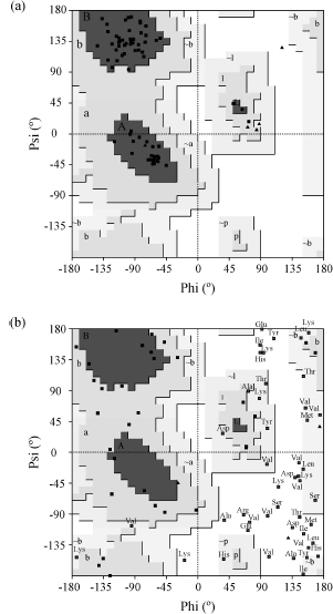
(a) Ubiquitin (PDB 1UBI), an X-ray structure at 1.8 Å: all but one of its 66 non-glycine, non-proline residues are in the core regions (labeled A, B, L), and they cluster tightly. Glycines are triangles. (b) An early NMR structure in which over a third of the residues lie in disallowed regions. Both plots are from PROCHECK.
Outliers, such as an unusual torsion angle, should not automatically be construed as errors. They may be genuine, for example as a result of strain in the conformation at an active site. The only way of verifying whether oddities are errors or merely oddities is by referring back to the original experimental data.
The core regions in these plots come from PROCHECK in the 1990s. Today's standard is MolProbity, whose contours come from about 100,000 residues in high-resolution structures; a good structure has about 98% of its residues in the "favored" region and almost none outside the "allowed" one. Predicted models get the same test: many outliers usually mean a backbone no protein could adopt.
Check yourself
A loop residue in a high-resolution crystal structure sits at (φ, ψ) = (+80°, +10°). What residue would you guess it is, and what would you suspect if it turned out to be a valine?
Reasoning
Glycine is the best guess: φ > 0 is open to glycine and nearly closed to everything else, with αL (around +57°, +47°) as a narrow exception for asparagine and aspartate. A valine there has its Cβ jammed against the backbone. In a high-resolution structure with clear density it could be real strain, perhaps holding an active site in shape. Otherwise it is a likely modeling error: check the electron density, and the residues on either side, which may have been traced out of register.
A designer wants to rigidify a flexible loop. Would replacing a glycine with alanine, or an alanine with proline, be the bigger restriction, and when could each replacement backfire?
Reasoning
Both shrink the loop's options, by different mechanisms. Gly → Ala removes the φ > 0 half of the plot that only glycine can use. Ala → Pro pins φ near −65° and removes a backbone N–H donor. Either backfires if the native loop needs what is taken away: a glycine sitting at φ > 0 cannot become alanine without strain, and a residue whose φ is far from −65°, or whose N–H makes a hydrogen bond, cannot become proline. So check the residue's current (φ, ψ) before choosing.
A predicted structure has every residue in an allowed region, but its loops look nothing like the crystal structure. Is the prediction validated?
Reasoning
No. The Ramachandran plot checks local stereochemistry, meaning each residue's own two angles. It says nothing about whether the chain's global fold, or the arrangement of its loops, is right. A model can be locally ideal and globally wrong. Comparing with the experimental structure (RMSD, or a contact-based score) or with the experimental data tests the fold. The plot only rules models out.