Reading the fine print
A structure file also says how sure it is, if you know where to look. The header gives resolution, R, and R-free for the whole entry; every atom carries an occupancy and a B factor; and atoms that were never seen are listed separately or simply missing. Read these before trusting a distance, a rotamer, or a binding pocket. The hard question comes at the end: is a fuzzy region fuzzy because the molecule moves, or because the data ran out?
Resolution
The resolution at which a structure is determined provides a measure of the amount of detail that can be discerned in the computed electron density map. The reflections at larger scattering angles in the diffraction pattern correspond to higher resolution information, coming as they do from crystal planes with a smaller interplanar spacing. The high-angle reflections tend to be of a lower intensity and more difficult to measure, and the greater the disorder in the crystal, the more of these high-angle reflections will be lost. Resolution relates to how many of these high-angle reflections can be observed, although the value actually quoted can vary from crystallographer to crystallographer, as there is no clear definition of how it should be calculated.
The resolution attainable for a given crystal depends on how well ordered the crystal is, that is, how close the unit cells throughout the crystal are to being identical copies of one another. A simple rule of thumb is that the larger the molecule, the lower will be the resolution of the data collected.
The figure below shows how the electron density for a single side chain improves as resolution increases. In general, side chains are difficult to make out at very low resolution (4 Å or lower), and the best that can be obtained is the overall shape of the molecule and the general locations of the regions of regular secondary structure. At 3 Å resolution, the path of a protein's chain can be traced through the density and at 2 Å, the side chains can be confidently fitted.
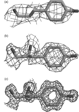
The most precise structures are the atomic resolution ones (from around 1.2 Å resolution up to around 0.9 Å). Here the electron density is so clear that many of the hydrogen atoms become visible, and alternative occupancies become more easily distinguishable. The resolution of X-ray structures in the PDB varies from atomic resolution structures to very low-resolution structures at around 4.0 Å, with a definite peak at around 2.0 Å.
Resolution is a length, and smaller is better: it is the smallest spacing between planes of atoms in the crystal whose reflections were measured, related to the scattering angle and the wavelength by Bragg's law, . To see what a resolution limit does to density, model each atom as a Gaussian blob of electrons whose width grows with (and with the atom's B factor, below), and add the blobs up. That is all the figure below does, for the tryptophan side chain of myoglobin's Trp 14 taken from the 1.0 Å entry 1A6M.
Code
import numpy as np
from primer import structure, display_widget

res = structure("1A6M")[0]["A"][14]
atoms = [a for a in res if a.element != "H"]
ring = np.array([res[n].coord for n in ("CG", "CD1", "CD2", "NE1", "CE2", "CE3", "CZ2", "CZ3", "CH2")])
center = ring.mean(axis=0)
_, _, axes = np.linalg.svd(ring - center)          # the first two axes span the plane of the indole rings
xy = (np.array([a.coord for a in atoms]) - center) @ axes[:2].T
bonds = [[i, j] for i in range(len(atoms)) for j in range(i)
         if np.linalg.norm(atoms[i].coord - atoms[j].coord) < 1.9]
display_widget(
    "density-map",
    "Trp 14 of myoglobin (1A6M), seen face-on to its two fused rings, with each atom smeared into a "
    "Gaussian whose width grows with the resolution $d$ and the B factor. The line is the contour a "
    "crystallographer would draw. Raise $d$ and the rings' holes close, the five-membered ring's first; "
    "by 3.5 Å the side chain is a featureless bulge you could fit in more than one orientation. This map "
    "is idealized, with perfect phases and no noise, so detail survives to somewhat worse resolution "
    "than in a real map, where aromatic ring holes usually close by about 1.5–2 Å.",
    atoms=[[round(float(x), 3), round(float(y), 3), a.element, a.get_id()] for (x, y), a in zip(xy, atoms)],
    bonds=bonds, resolution=2.0, b=20,
)
Trp 14 of myoglobin (1A6M), seen face-on to its two fused rings, with each atom smeared into a Gaussian whose width grows with the resolution and the B factor. The line is the contour a crystallographer would draw. Raise and the rings' holes close, the five-membered ring's first; by 3.5 Å the side chain is a featureless bulge you could fit in more than one orientation. This map is idealized, with perfect phases and no noise, so detail survives to somewhat worse resolution than in a real map, where aromatic ring holes usually close by about 1.5–2 Å.
Cryo-EM maps also quote a resolution, estimated differently (from how well maps built from two halves of the particles agree), and it varies across a map. NMR structures have no resolution at all.
R and R-free
The R-factor is a measure of the difference between the structure factors (the Fourier coefficients of lesson 6.1, one per reflection) calculated from the model and those obtained from the experimental data. Typically, for protein and nucleic acid structures, values quoted for the R-factor tend to be around 0.20 (or equivalently, 20%). Values in the range 0.40–0.60 can be obtained from a totally random structure, so structures with such values are unreliable.
As a reliability measure, however, the R-factor is in itself somewhat unreliable. It is quite easily susceptible to manipulation, either deliberate or unwary, during the refinement process, and so models with major errors can still have reasonable-looking R-factors. For example, the fully refined structure of ferredoxin I was deposited in 1981 as PDB code 2FD1, with a quoted resolution of 2.0 Å and an R-factor of 0.262. Due to the incorrect assignment of the crystal space group,The space group is the set of symmetry operations (rotations, screw axes, mirrors for non-biological crystals) that map copies of the molecule onto each other within the crystal. There are 230 in all, and only 65 are possible for crystals of L amino acids, since a mirror would turn them into D. this structure turned out to be completely wrong. The replacement structure, having the correct fold, was deposited as 3DF1 in 1988, at 2.7 Å with an R-factor of 0.35. On the face of it, comparison of the resolution and R-factor parameters would lead one to believe the first of the two structures to be the more reliable! The reason why an R-factor as low as 0.262 was achieved for a totally incorrect structure was that the coordinates included 344 water molecules, many extending far out from the protein molecule itself, a large number for a protein of only 107 residues. A well-known rule of thumb suggests that a reasonable number of waters is roughly one water molecule for each protein residue at around 2 Å resolution; at 1.0 Å one can reasonably expect 1.6–1.7 waters per residue. One can always fit a model, however wrong, to the experimental data and obtain a reasonable R-factor if there is an excess of parameters over observations.
A more reliable reliability factor is Brünger's free R-factor, or Rfree. It is calculated in the same way, but using only a small fraction of the experimental data, typically 5–10%. This fraction, known as the test set, is excluded from the structure refinement procedure that uses the remaining 90–95% of the data, or working set. Thus, unless there are correlations between the data in the test and working sets, the Rfree provides an independent measure of the fit of the model to the data and cannot be biased by the refinement process. The value of Rfree will tend to be larger than the R-factor; any value above 0.40 should be treated with caution.
In symbols, , summed over the working reflections for R and over the test reflections for R-free: a training error and a validation error. A gap between them much wider than about 0.05 suggests overfitting, and a common rule of thumb for a good structure is an R-free near a tenth of the resolution (about 0.20 at 2 Å). R-free dates from 1992, so older entries such as 1UBQ (1987, R = 0.176) and 4HHB (1984) don't report one. The water rule checks out on the anchors: 1UBQ at 1.8 Å has 58 waters for 76 residues, and 7RSA at 1.26 Å has 188 for 124.
A commonly used rule of thumb for selecting reliable structures for analyses where reasonably accurate models are required is to choose those models that have a quoted resolution of 2.0 Å or better, and an R-factor of 0.20 or lower. These criteria will give structures that are likely to be reasonably reliable down to the conformations of the side chains and local atom-atom interactions. Of course, the selection criteria depend on the type of analysis required. For some analyses, only atomic resolution structures (1.2 Å or better) will do, as in the accurate derivation of side chain torsional conformers. For other types of analysis, structures solved down to 3 Å may be good enough, as in any comparison of protein folds. Often this rule of thumb is supplemented by a check on the year when the structure was determined, since techniques have improved markedly since the early days of the 1960s and 1970s.
B factors
Every atom in an X-ray model carries a B factor (also called the temperature factor or atomic displacement parameter), in Ų. It is the width of the Gaussian smear the model uses for that atom: if the atom's position fluctuates with mean-square displacement along any one direction, then
So Ų means a root-mean-square displacement of 0.50 Å along each axis, and Ų means 1.0 Å, two-thirds of a C–C bond. The "displacement" collects everything that makes copies of an atom differ across the crystal and the exposure: thermal vibration, static disorder (different molecules frozen in slightly different places), defects in the lattice, and errors in the model. Refinement settings and restraints shift B factors too, so compare them within a structure, not across entries.
A direct, albeit merely qualitative, way of determining the precision of a given atom's coordinates is to look at its associated B-factor. B-factors are closely related to the positional errors of the atoms, although the relationship is not a simple one that can be easily formulated. It is safe to say, however, that atoms in a structure with the largest B-values will also be those having the largest positional uncertainty. So if high levels of precision are required in your analysis, leave out the atoms having the highest B-factors. As a rule of thumb, atoms with B-values in excess of 40 are often excluded as being too unreliable. Similarly, if atoms in your region of interest, such as an active site, are all cursed with high B-factors then your region of interest is not well determined, and you will either need to be careful about the conclusions you draw from it, or else seek out a different structural model of the same protein where the region is better defined.
Ubiquitin's Cα B factors, residue by residue, against the secondary structure in the file's HELIX and SHEET records:
import matplotlib.pyplot as plt
from primer import fetch

ubq = structure("1UBQ")[0]["A"]
residues = [r for r in ubq if r.id[0] == " "]
numbers = [r.id[1] for r in residues]
b_ca = [r["CA"].bfactor for r in residues]

def ranges(record):
    """(start, end) residue numbers of each HELIX or SHEET record (legacy PDB columns)."""
    cols = {"HELIX": (21, 25, 33, 37), "SHEET": (22, 26, 33, 37)}[record]
    return [(int(l[cols[0]:cols[1]]), int(l[cols[2]:cols[3]]))
            for l in open(fetch("1UBQ")) if l.startswith(record)]

fig, ax = plt.subplots(figsize=(6.4, 2.8))
for start, end in ranges("HELIX"):
    ax.axvspan(start - 0.5, end + 0.5, color="#eb6834", alpha=0.18, lw=0)
for start, end in ranges("SHEET"):
    ax.axvspan(start - 0.5, end + 0.5, color="#2a78d6", alpha=0.18, lw=0)
ax.plot(numbers, b_ca, color="#333333", lw=1.5)
ax.set_xlabel("residue number")
ax.set_ylabel("Cα B factor (Ų)")
ax.text(1, 33, "orange: helix, blue: strand", fontsize=9, color="#555555")
plt.show()
print(f"Cα B factors range from {min(b_ca):.1f} to {max(b_ca):.1f} Ų; residues 72–76: "
      + ", ".join(f"{b:.0f}" for b in b_ca[71:]))
Cα B factors range from 3.5 to 36.2 Ų; residues 72–76: 26, 31, 35, 36, 36
The strands and the helix sit low, and the C-terminal tail (Leu–Arg–Gly–Gly, residues 73–76) climbs to over 35 Ų. That tail is the end that enzymes attach to other proteins, and in solution it is flexible. Seen in 3D:
Ubiquitin (1UBQ) colored by B factor. The packed core is pale and the C-terminal tail, pointing away at one end, is dark.
Open 1UBQ in Mol*An AlphaFold file uses the same column for pLDDT, a confidence on a 0–100 scale where high is good, the opposite sense of a B factor. A pipeline that reads pLDDT as a B factor (some older ones do) gets every residue backwards.
Alternate conformations, occupancy, and absences
Occupancy and alternate locations describe atoms that are in more than one place. If the density supports two positions for a side chain, the model gives both, labeled A and B in the altloc field, with occupancies that add up to about 1. The 1.26 Å RNase A model 7RSA has several:
rnase = structure("7RSA")[0]["A"]
for residue in rnase:
    split = [a for a in residue if a.is_disordered() and a.element != "H"]
    if split:
        occ = {alt: round(atom.occupancy, 2) for alt, atom in split[0].child_dict.items()}
        print(f"{residue.get_resname()} {residue.id[1]:>3}: {len(split)} atoms in two positions, occupancies {occ}")
GLN  11: 5 atoms in two positions, occupancies {'A': 0.66, 'B': 0.33}
SER  32: 2 atoms in two positions, occupancies {'A': 0.67, 'B': 0.33}
ASN  34: 4 atoms in two positions, occupancies {'A': 0.33, 'B': 0.67}
VAL  43: 3 atoms in two positions, occupancies {'A': 0.4, 'B': 0.6}
SER  50: 2 atoms in two positions, occupancies {'A': 0.67, 'B': 0.33}
LYS  61: 5 atoms in two positions, occupancies {'A': 0.5, 'B': 0.5}
ASN  67: 4 atoms in two positions, occupancies {'A': 0.67, 'B': 0.33}
SER  77: 2 atoms in two positions, occupancies {'A': 0.67, 'B': 0.33}
ASP  83: 4 atoms in two positions, occupancies {'A': 0.5, 'B': 0.5}
ARG  85: 7 atoms in two positions, occupancies {'A': 0.5, 'B': 0.5}
LYS  91: 5 atoms in two positions, occupancies {'A': 0.5, 'B': 0.5}
LYS  98: 5 atoms in two positions, occupancies {'A': 0.5, 'B': 0.5}
LYS 104: 5 atoms in two positions, occupancies {'A': 0.5, 'B': 0.5}
Gln 11's side chain sits in one position in about two-thirds of the molecules and another in one-third; several lysines split 50/50. At high resolution the model starts recording how the ~10¹³ molecules in the crystal differ from one another.
Within an individual structure there can be wide variability in local accuracy. Regardless of resolution, most structures have a few parts disordered enough that they are not visible at all in a crystallographic electron-density map (or have no observable NMR restraints), and other parts only weakly tied to data. In some cases (especially at chain termini), the coordinates of those atoms will be omitted in the data bank file, but more often disordered areas are indicated by a high crystallographic B-factor or by highly divergent conformations in an NMR ensemble. If a particular part of a structure is important to the question being asked, these telltale signs should always be heeded: they indicate that the local conformation is highly uncertain, either because of molecular motions or because of problems with the data. Regions of locally ambiguous data not only produce a higher level of random errors but also quite often result in systematic errors of interpretation that move atoms by several ångströms.
Absences come in several kinds, and each is recorded somewhere:
| What's absent | Where the file records it | Example |
|---|---|---|
| Residues in the sequence but not in the model, usually termini or long loops | REMARK 465; _pdbx_unobs_or_zero_occ_residues in mmCIF | the EGFR kinase entry 1M17 lacks residues 666–671, 965–976, and 996–998 |
| Side-chain atoms without density, often cut back to Cβ | REMARK 470 | surface lysines and glutamates |
| Atoms kept at zero occupancy, placed without supporting density | occupancy column 0.00 | every atom of Glu 725 in 1M17, with B near 118 Ų |
| Hydrogens, and all but the ordered water | nowhere: the model simply lacks them | thousands of water molecules surround a protein; a model lists a few hundred at most |
A program that ignores the occupancy column will treat 1M17's Glu 725 as real.
Validation: comparing a model with what is normal
Given that all structural models contain some degree of error, a large class of checks examines a model's geometry, stereochemistry, and other structural properties. These checks compare a given protein or nucleic acid structure against what is already known about these molecules. The "knowledge" comes from high-resolution structures of small molecules plus systematic analyses of the existing protein and nucleic acid structures in the PDB. The advantage of such tests of "normality" is that they do not require access to the original experimental data, so any 3D structure, whether experimentally determined, or the result of homology modeling, molecular dynamics, threading (fitting a sequence onto known folds) or blind guesswork, can be checked.
One point needs stressing. The majority of the checks compare a given structure's properties against what is the "norm." Outliers, such as an excessively long bond length or an unusual torsion angle, should not be construed as errors. They may be genuine, for example as a result of strain in the conformation, say, at the active site. The only way of verifying whether oddities are errors or merely oddities is by referring back to the original experimental data. Having said that, if a single structure exhibits a large number of outliers and oddities, then it probably does have problems.
Of special importance in validation are independent criteria, not explicitly part of the target function optimized by the structure refinement process, because the new information makes their deviations more sensitive and robust indicators of problems. The two classic indicators are (1) the backbone φ, ψ, or "Ramachandran" plot, since joint φ, ψ values are not in usual target functions, and (2) the free R-factor.
Lesson 3.2 covered the Ramachandran check. The validation report the PDB attaches to every entry adds an all-atom contact check, the clashscore: the number of serious steric overlaps (atoms closer than their radii allow by 0.4 Å or more) per 1,000 atoms, with hydrogens added first. It also reports the percentage of Ramachandran and side-chain outliers and how well each residue fits the density, and it places each number on a percentile slider against other entries of similar resolution.
Of all the errors, the most serious are those where the model is, essentially, completely wrong, such as when the trace of the protein chain follows the wrong path through the electron density, resulting in a completely incorrect fold. Less serious are frame shift errors, although they can often result in a significant part of the model being incorrect. These errors occur where a residue is fitted into the electron density that belongs to the next residue. The frame shift persists until a compensating error is made when two residues are fitted into the density belonging to a single residue. These mistakes often occur in loop regions, and almost exclusively at low resolution (3 Å or lower).
Typically, the majority of the models deposited in the PDB will be essentially correct. A surprising result from one study was that some types of errors that are relatively easy to detect and fix were still turning up in newly released PDB entries: 3.6% of the amino acids contained an error of some kind. The most common errors were His/Asn/Gln side chain flips. These side chains are symmetrical in terms of shape and so will fit their electron density equally well when rotated by 180°. However, their chemical properties are not symmetrical and, in general, one orientation will result in a better hydrogen-bonding network than the other. This can be critical when the side chain in question is part of a catalytic or binding site.
The flip problem is one more consequence of invisible hydrogens. In histidine's ring, and at the ends of asparagine and glutamine, a nitrogen and a carbon (or an oxygen) have nearly the same number of electrons, so the density can't tell which is which; only the hydrogen-bonding pattern can.
NMR models have their own fine print
The theory of NMR spectroscopy does not provide a means of obtaining uncertainties for atomic coordinates directly from the experimental data, so estimates of a structure's accuracy and precision have to be obtained by more indirect means. It is difficult to distinguish whether the multiplicity of models in an ensemble reflects real motion within the molecules or simply results from insufficient experimentally derived restraints. The agreement of NMR models with the NMR data is measured by the agreement between the distance and angular restraints applied during refinement and the corresponding distances and angles in the final models. However, the errors associated with the original experimental data are sufficiently large that it is almost always possible to generate models that do not violate the restraints, or do so only slightly.
Traditionally, the "quality" of a structure solved by NMR has been measured by the root-mean-squared deviation (RMSD) across the ensemble. Regions with high RMSD values are those that are less well defined by the data. However, the values obtained are rather dependent on the procedure used to generate and select models for deposition. An experimentalist choosing the "best" few structures from a much larger draft ensemble can obtain very misleading statistics: the "best" few structures may, in effect, be the same solution with minor variations, so the RMSD values will be small.
Noise or motion?
Every signal in this lesson can mean two things, and the file alone rarely says which.
| What you see | Could mean the molecule moves | Could mean the data ran out |
|---|---|---|
| High B factors | the atoms vibrate or switch between states | static disorder, lattice defects, or an error in the model |
| Missing residues | a flexible loop or terminus | poor crystals, or a region cut out of the construct |
| Two alternate conformations | the side chain really visits both | (rarely) a fitting compromise for ambiguous density |
| Spread in an NMR ensemble | motion in solution | too few restraints in that region |
| Low pLDDT in a prediction | intrinsic disorder | too few related sequences for the predictor |
Telling them apart takes evidence from outside the one model: a second crystal form, an NMR relaxation experiment, a molecular dynamics simulation, or a functional assay. And even a flawless model shows one state: kinases have active and inactive forms, hemoglobin has T and R, and the entry you downloaded caught one of them under one set of conditions.
Check yourself
Two crystal structures of the same enzyme are available: one at 1.6 Å with R/R-free = 0.18/0.29, and one at 2.1 Å with R/R-free = 0.19/0.23. Which would you choose to measure hydrogen-bond distances in the active site, and why?
Reasoning
Probably the 2.1 Å structure. The 1.6 Å model's gap between R and R-free (0.11) is large: it fits the working reflections much better than the held-out ones, which is the signature of overfitting. Its better nominal resolution doesn't help if the model isn't supported by the data. The 2.1 Å model's gap (0.04) and R-free near a tenth of its resolution look healthy. Before measuring, also check the B factors and occupancies of the active-site atoms in whichever model you pick.
A loop in a 2.0 Šcrystal structure has B factors around 70 Ų while the core sits near 15 Ų. A colleague concludes the loop is "highly dynamic in the cell." What else could explain the B factors, and what would make you more confident in the colleague's reading?
Reasoning
B factors absorb static disorder (the loop frozen in different positions in different unit cells), lattice defects, and modeling errors, not only motion. If the loop also touches a neighboring molecule in some unit cells and not others, packing could be the cause. More confidence would come from independent evidence: high B in other crystal forms of the same protein, missing or weak density in several structures, spread in an NMR ensemble or low order parameters from NMR relaxation, or motion in a molecular dynamics simulation.
You are building a training set of protein–ligand complexes and want every ligand to be really there. Which columns and records would you filter on, and why?
Reasoning
Occupancy (drop or flag ligands with occupancy well below 1, including 0.00), B factors of the ligand relative to the protein atoms around it (ligand B far above its neighbors suggests weak density), and the entry's resolution and R-free. Ideally also the per-ligand density fit in the validation report. A ligand can be present in the coordinates and still be poorly supported by the data, since a modeler chose to place it.
An AlphaFold model's B-factor column reads 35 for residues 1–40 and 92 for residues 41–200. A script written for crystal structures flags residues 41–200 as "highly flexible." What went wrong?
Reasoning
The script read pLDDT as a B factor. In an AlphaFold file, high values mean high confidence, so residues
41–200 are the confident, probably well-folded domain, and residues 1–40 are the low-confidence and likely
disordered part. The file format is the same as an X-ray entry's, so the script had to check the
provenance (the header or _exptl.method) before interpreting the column.