Models, not photographs
A structure file lists atoms with x, y, z coordinates, and nobody has ever seen those atoms. The coordinates are a model fitted to indirect measurements, and each method (X-ray crystallography, NMR, cryo-EM) leaves its own fingerprints on the model. Predicted structures go one step further: no measurement of the molecule at all.
Keep three things apart: the measurements (diffraction spots, NMR spectra, electron micrographs), the model fitted to them (coordinates plus numbers saying how well they fit), and the image a program draws from the model (lesson 6.4). A coordinate file holds only the model.
In X-ray crystallography, programs take the diffraction data obtained from a purified protein crystal, generate electron density maps, build the molecular model, and refine the model. The result of this process is a file containing the 3D orthogonal coordinates (x, y, z) of the refined molecule.
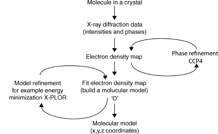
Models from X-ray crystallography
Why X-rays, and why a crystal? To see two things as separate you need light whose wavelength is no longer than the gap between them. Visible light has wavelengths around 500 nm, thousands of times longer than a 1.5 Å bond, while the X-rays used for proteins are about 1 Å. Two obstacles remain: no lens can focus X-rays into an image, and a single molecule scatters far too little to detect. A crystal fixes the second. It is a solid in which one small box of molecules, the unit cell, repeats in all three directions like tiles. Waves scattered by all those identical copies reinforce each other in a few directions and cancel in all the others (diffraction), so the scattered X-rays collect into sharp spots. With no lens, the image has to be computed from the spots. X-rays scatter from electrons, so what you compute is the electron density , the number of electrons per ų at each point: high where atoms are, with roughly one peak per non-hydrogen atom, and near zero between them.
A typical protein crystal holds about copies, all scattering in step. Each spot, or reflection, is one Fourier coefficient of the electron density, where is a triple of integers that labels the spot: (with the unit cell's volume). Each is a complex number with an amplitude and a phase. The detector measures only the intensity, , so the phases are lost. This is the phase problem. How much do the missing phases matter? Swap them between two molecules and see which molecule you get back:
import numpy as np
import matplotlib.pyplot as plt
from primer import structure

def heavy_atoms(pdb_id):
    """Non-hydrogen, non-water atoms, centered and turned so the molecule's widest extent faces us."""
    xyz = np.array([a.coord for a in structure(pdb_id)[0].get_atoms()
                    if a.element != "H" and a.get_parent().get_resname() != "HOH"])
    xyz = xyz - xyz.mean(axis=0)
    _, _, axes = np.linalg.svd(xyz, full_matrices=False)
    return xyz @ axes.T

def density_image(xyz, size=96, step=1.0, blur=1.5):
    """Project atoms onto a size × size grid (step Å per pixel), each blurred into a Gaussian."""
    edges = (np.arange(size + 1) - size / 2) * step
    counts, _, _ = np.histogram2d(xyz[:, 0], xyz[:, 1], bins=[edges, edges])
    k = np.fft.fftfreq(size, d=step)
    kx, ky = np.meshgrid(k, k, indexing="ij")
    gaussian = np.exp(-2 * (np.pi * blur) ** 2 * (kx**2 + ky**2))   # blurring is a product in Fourier space
    return np.real(np.fft.ifft2(np.fft.fft2(counts) * gaussian))

trna, hb = density_image(heavy_atoms("1EHZ")), density_image(heavy_atoms("4HHB"))
F_trna, F_hb = np.fft.fft2(trna), np.fft.fft2(hb)
swap1 = np.real(np.fft.ifft2(np.abs(F_trna) * np.exp(1j * np.angle(F_hb))))
swap2 = np.real(np.fft.ifft2(np.abs(F_hb) * np.exp(1j * np.angle(F_trna))))

fig, axs = plt.subplots(1, 4, figsize=(10, 2.9))
titles = ["tRNA (1EHZ)", "hemoglobin (4HHB)", "tRNA amplitudes,\nhemoglobin phases", "hemoglobin amplitudes,\ntRNA phases"]
for ax, img, title in zip(axs, [trna, hb, swap1, swap2], titles):
    ax.imshow(img.T, origin="lower", cmap="Blues")
    ax.set_title(title, fontsize=10)
    ax.axis("off")
plt.show()
Each swapped image looks like the molecule that supplied the phases, not the amplitudes. The detector throws away exactly the half of the data that carries the picture, so crystallographers get phases elsewhere: from a few heavy atoms whose contributions can be located on their own (often selenium, built in by growing the protein on selenomethionine, methionine with its sulfur replaced by selenium), or from a similar known structure.
The method of molecular replacement is commonly used to solve structures for which a homologous structure is already known. The method attempts to locate a molecule or fragments of a molecule, whose structure is known, in the unit cell of an unknown structure for which experimental data are available. To make the problem tractable, it has traditionally been broken down into two consecutive three-dimensional search problems: a search to determine the rotational orientation of the model followed by a search to determine the translational orientation for the rotated model.
Molecular replacement is now the most common route, and since 2021 the search model is often an AlphaFold prediction. With starting phases you compute a first map, build a chain into it, and refine.
In general, the atomic model obtained by automatic or manual methods contains some errors and must be optimized to best fit the experimental diffraction data and prior chemical information. However, the refinement of macromolecular structures is often difficult. First, the data to parameter ratio is low, creating the danger of overfitting the diffraction data. This results in a good agreement of the model to the experimental data even when it contains significant errors. Therefore, the apparent ratio of data to parameters is often increased by incorporation of chemical information, that is, bond length and bond angle restraints obtained from ideal values seen in high-resolution structures. Second, the initial model often has significant errors, often due to the limited quality of the experimental data or a low level of homology between the search model and the true structure in molecular replacement. Third, local (false) minima exist in the target function. Fourth, model bias in the electron density maps complicates the process of manual rebuilding between cycles of automated refinement.
Cross-validation, in the form of the free R-value, can be used to detect overfitting.
In machine-learning terms, refinement fits thousands of parameters, the geometric restraints are a prior, and R-free is the validation error on held-out reflections (lesson 6.2). The result is an average over ~10¹³ molecules, usually frozen to about 100 K. Hydrogen has a single electron and scatters too weakly to see, so when an X-ray model lists hydrogens, refinement placed them where chemistry says they belong.
A refined X-ray model holds more than coordinates. Rubredoxin, solved by both X-ray crystallography and NMR, shows what each method deposits:
The figure below shows two different interpretations of the same protein given by the two methods. The models are of the protein rubredoxin with a bound metal ion held in place by four cysteines. Both can be found in the PDB: the X-ray model (PDB code 1IRN) has a zinc as its metal ion while in the NMR model (1BFY), the metal ion is iron.
Panel (a) is a representation of the protein model as obtained by X-ray crystallography. The components are the x-, y-, z-coordinates, B-factors and occupancies of all the individual atoms in the structure. These parameters, together with the theory that explains how X-rays are scattered by the electron clouds of atoms, aim to account for the observed diffraction pattern. The x-, y-, z-coordinates define the mean position of each atom while its B-factor and occupancy aim to model its apparent disorder about that mean. This disorder may be the result of variations in the atom's position in time, due to the dynamic motions of the molecule, or variations in space, corresponding to differences in conformation from one location in the crystal to another, or both. The higher the atom's disorder, the more "smeared out" its electron density. B-factors model this apparent smearing around the atom's mean location; at high resolution a better fit can often be obtained by assuming the B-factors to be anisotropic, as represented by the ellipsoids in panel (a). Occasionally, the data can be explained better by assuming that certain atoms can be in more than one place, say, due to alternative conformations of a particular side chain (the arrows showing the two positions of the glutamate side chain). The atom's occupancy defines how often it is found in one conformation and how often in another (here, 56% and 44%).
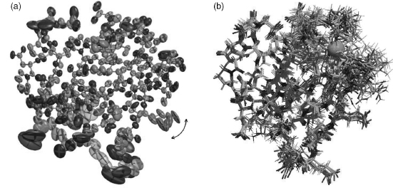
Models from NMR spectroscopy
NMR (nuclear magnetic resonance) listens to atomic nuclei instead of electrons. Some nuclei, including hydrogen's, behave like tiny bar magnets, a property called spin. In a strong magnetic field (the physics of a hospital MRI scanner) they absorb radio waves at a frequency that shifts slightly with their chemical surroundings. That chemical shift gives each hydrogen in a protein its own peak in the spectrum, once someone works out which peak belongs to which atom. Two hydrogens close in space also pass magnetization to each other, the nuclear Overhauser effect (NOE), and the transfer weakens steeply with distance. An NOE between two hydrogens says they lie within about 5–6 Å of each other.
Generally, the sample of protein or nucleic acid is in solution, rather than in crystal form, which means that molecules that are difficult to crystallize can often be solved by NMR instead. The most numerous, but often least precise, data are from Nuclear Overhauser Effect Spectroscopy (NOESY) experiments where the intensities of particular signals correspond to the separations between spatially close protons (< 6 Å) in the structure.
The proton separations obtained from the experimental data are converted into distance and angular restraints that are used to generate models of the structure that are consistent with these restraints. The most commonly used are molecular dynamics based simulated annealing procedures similar to those used in X-ray structure refinement. The end result is not a single model, but rather an ensemble of models that are all consistent with the given restraints.
The reasons for generating an ensemble of structures from NMR data are twofold. Firstly, the NMR data are relatively less precise and less numerous than experimental restraints from X-rays, so a diversity of structures are consistent with them. Secondly, the molecules may genuinely possess heterogeneity in solution. Ensembles deposited in the PDB typically comprise 20 models. One of the models may be designated the "representative" of the whole ensemble, usually the structure that differs least from all the others.
Turning those distances into coordinates is a classic computational-geometry problem, and a hard one.
Nuclear Overhauser Enhancement (NOE). The NOE is a consequence of dipole-dipole coupling and cross-relaxation between different nuclear spins, and is used to measure the distance between atoms (usually protons) in proteins. The relation between the observed NOE intensity and the distance is ideally .
Distance geometry problem. Let where denote the coordinates of atoms . The distance geometry problem is to find coordinates such that the given distance constraints are all satisfied.
- If the exact distances between all pairs of atoms are known, the problem can be solved in time by using the singular value decomposition.
- Given only a subset of the distances, the problem becomes difficult to solve: it is (strongly) NP-hard.
- Because of the noise from experimental data, we may only get lower and upper bounds on the distances. Even finding an approximate solution is still NP-hard.
NMR data are case 3, and sparse besides: noisy upper bounds, only between hydrogens within about 6 Å of each other. Many structures satisfy them, which is why the output is an ensemble. Ubiquitin's 1D3Z is one of the most precisely determined NMR structures; below are its ten models. NMR models include their hydrogens, because NMR observes them.
The ten models of 1D3Z (ubiquitin by NMR) superposed as Cα traces, colored from the N-terminus (blue) to the C-terminus (red). The core agrees to a fraction of an ångström; the last few residues of the C-terminal tail fan out.
Open 1D3Z in Mol*Models from cryo-EM
Cryo-electron microscopy (cryo-EM) takes actual pictures, with electrons instead of light. Electrons have wavelengths far below an ångström and, unlike X-rays, can be focused by magnetic lenses, so an electron microscope forms real images. The catches are that the sample must sit in a vacuum and that electrons wreck biological molecules. The answer is to freeze a thin film of the solution so fast that the water becomes a glass rather than ice crystals (vitrified ice), and to image it with very few electrons. Each copy of the molecule caught in the ice, lying in some random orientation, is a particle.
Each sample must be prepared in a relatively homogeneous, aqueous form. This specimen is then rapidly frozen (vitrified) as a thin film, transferred to the electron microscope and imaged under low-dose conditions (less than about 50 electrons per Ų).
An electron micrograph consists of two-dimensional projections of a three-dimensional object. To retrieve its three-dimensional structure, sufficiently sampled angular views of the object need to be aligned and combined. There are three basic tasks. First, images of the object must be obtained in a sufficient number of orientations; for single particles, this comes from their random orientations in the ice. Second, the orientation and center of the object needs to be determined. Iterative refinement of these parameters is usually carried out by cross-comparison between different images or by projection images of preliminary models. Third, image shifts must be applied computationally to bring all views of the object to a common origin. Only then a three-dimensional reconstruction can be calculated.
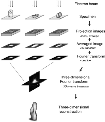
The low dose is the difficulty: electrons destroy molecules, so each particle image is mostly noise. Averaging aligned images of the same view improves the signal-to-noise ratio by , because the noise is independent between images and the signal isn't:
rng = np.random.default_rng(0)
view = density_image(heavy_atoms("4HHB"), size=80)
view /= view.std()
particle = lambda: view + rng.normal(0, 6, view.shape)   # noise six times the signal

fig, axs = plt.subplots(1, 5, figsize=(10, 2.4))
for ax, n in zip(axs, [1, 10, 100, 1000]):
    ax.imshow(np.mean([particle() for _ in range(n)], axis=0).T, origin="lower", cmap="gray")
    ax.set_title(f"average of {n}", fontsize=10)
axs[4].imshow(view.T, origin="lower", cmap="gray")
axs[4].set_title("noise-free", fontsize=10)
for ax in axs:
    ax.axis("off")
plt.show()
Until about 2013, cryo-EM maps rarely beat 7 Å. Direct electron detectors and better software changed that (the 2017 Nobel Prize in Chemistry went to cryo-EM), and most single-particle maps now land between 2.5 and 4 Å, with the best near 1.2 Å. A model is built into the map as in crystallography, with three differences. Resolution varies across a map: the rigid core averages well and flexible arms blur, so the global figure (from comparing maps built from two halves of the data) can hide a much worse local resolution at the site you care about. Particles in different conformations can be sorted into separate maps, each a real state of the molecule. And the method works best on large assemblies such as ribosomes, channels, and viral capsids, while proteins under about 50 kDaA dalton (Da) is the mass of a hydrogen atom, near enough. An average amino-acid residue weighs about 110 Da, so 50 kDa is roughly 450 residues; ubiquitin is 8.6 kDa. give too little contrast to align. Release counts in the PDB show how fast the field moved:
import json
import urllib.request

def entries(method, year):
    """Number of PDB entries released in a year whose experimental method is `method` (RCSB search API)."""
    rule = lambda attr, op, val: {"type": "terminal", "service": "text",
                                  "parameters": {"attribute": attr, "operator": op, "value": val}}
    query = {"query": {"type": "group", "logical_operator": "and", "nodes": [
                 rule("exptl.method", "exact_match", method),
                 rule("rcsb_accession_info.initial_release_date", "range",
                      {"from": f"{year}-01-01", "to": f"{year}-12-31",
                       "include_lower": True, "include_upper": True})]},
             "return_type": "entry", "request_options": {"return_counts": True}}
    req = urllib.request.Request("https://search.rcsb.org/rcsbsearch/v2/query",
                                 data=json.dumps(query).encode(), headers={"Content-Type": "application/json"})
    with urllib.request.urlopen(req, timeout=60) as r:
        return json.load(r)["total_count"]

years = range(2000, 2026)
methods = {"X-ray": "X-RAY DIFFRACTION", "cryo-EM": "ELECTRON MICROSCOPY", "NMR": "SOLUTION NMR"}
counts = {label: [entries(m, y) for y in years] for label, m in methods.items()}
for label in methods:
    print(f"{label:>7}: {counts[label][0]:>6} entries released in 2000, {counts[label][-1]:>6} in 2025")

fig, ax = plt.subplots(figsize=(6.4, 3.2))
for label, ys in counts.items():
    ax.plot(list(years), ys)
    ax.annotate(label, (2025, ys[-1]), xytext=(4, 0), textcoords="offset points", va="center")
ax.set_ylabel("entries released per year")
ax.set_xlim(2000, 2029)
plt.show()
  X-ray:   2231 entries released in 2000,  10083 in 2025
cryo-EM:     11 entries released in 2000,   7198 in 2025
NMR: 370 entries released in 2000, 225 in 2025Models with no measurement behind them
Particular skepticism should be reserved for models that are not directly based on any experimental measurement. Homology models rely on the fact that proteins sharing high sequence identity tend to have very similar overall 3D structures; proteins sharing a sequence identity greater than around 35% will have essentially the same fold. This makes it possible to generate a model of the 3D structure of a given protein based on the 3D model of a closely related protein. Even where the model is a good one, one needs to be cautious about taking the model's atomic positions at face value as they do not represent positions based on any experimental data. Any experimental errors in the template model will not only be propagated into the homology model but even exacerbated in the process.
Until 2020, structure prediction without a close template rarely produced accurate models. AlphaFold 2 (2021) and its successors predict many single domains close to experimental accuracy, and the AlphaFold Database holds over 200 million predicted structures, about one for every known protein sequence. They are written in the same PDB and mmCIF formats, line for line, as experimental models, so the file format can't tell you whether a coordinate was measured; only the metadata can. In an AlphaFold file the B-factor column holds the model's own per-residue confidence, pLDDT (0–100), instead of atomic smearing in Ų:
AlphaFold's prediction for human p53 (UniProt P04637), colored by pLDDT. The DNA-binding domain in the middle (residues ~94–292) and the small tetramerization domain (~325–355) are confident. The long N- and C-terminal stretches are low-confidence, correctly: those regions are intrinsically disordered (lesson 3.5).
Open AF-P04637 in Mol*AlphaFold files come with a second score, PAE (predicted aligned error): for each pair of residues, the expected error in one residue's position when the model is superimposed on the other. Low PAE between two domains means their relative placement is trustworthy, which pLDDT alone can't tell you.
A predicted model, however accurate, is a hypothesis built from patterns in other proteins' structures, with no measurement of the protein it describes.
When models and other data disagree
Several structures of one protein, or a structure and other experiments, often disagree.
One example is the noncrystallographic structural data on the two subunits of the bacterial ribosome (the machine that builds proteins) stored in RiboWEB, a knowledge base of more than 8000 structural and functional observations about the bacterial ribosome. RiboWEB has been used to assess the compatibility of the published ribosomal crystal structures with over 1000 proximity measurements from cross-linking, chemical protection, and labeling experiments.Experiments that report which parts of a molecule sit close together, for example by chemically tying neighbors to each other, or by seeing which parts a bound partner shields from a reagent. Incompatibilities between these data and the crystal structures may suggest artifactual data or (more usefully) may suggest areas of important dynamic motion for the ribosome.
A disagreement can be an artifact. Crystal packing can pin a loop, a construct (the version of the protein the experimenters actually made) trimmed so that it crystallizes can lack a domain that normally holds a helix in place, and sparse NMR restraints or weak cryo-EM density leave regions undetermined. Or it can be real: a different ligand, pH, or binding partner, or two states the protein really adopts. Hemoglobin's T and R forms are separate entries, 4HHB and 1HHO.
| X-ray crystallography | Solution NMR | Cryo-EM | Prediction | |
|---|---|---|---|---|
| Measures | diffraction amplitudes (phases lost) | NOE distances, couplings, shifts | noisy 2D projections of single particles | nothing about this molecule |
| Model fitted to | electron density | distance and angle restraints | a reconstructed 3D map | patterns learned from the PDB |
| Deposits | one model, with alternate conformations | an ensemble of 10–20 | one model per map | one model per sequence |
| Hydrogens | rarely, and placed | yes | rarely, and placed | none |
| Quality numbers | resolution, R, R-free, B | restraint violations, ensemble spread | global and local resolution | pLDDT, PAE |
Check yourself
A colleague says, "The file has hydrogens, so this must be an NMR structure." Is that a safe inference?
Reasoning
No. NMR models contain hydrogens because NMR observes them, but hydrogens also appear in high-resolution
X-ray models, placed by refinement at ideal positions (the 1.26 Å RNase A entry 7RSA lists 919 of them),
and in any file a program has processed, since many tools add hydrogens before simulation or docking.
The method is recorded explicitly (EXPDTA in the legacy format, _exptl.method in mmCIF).
In the phase-swap experiment the image followed the phases, not the amplitudes. Why does that make molecular replacement with a similar protein risky, and what does R-free protect against?
Reasoning
The first map's phases come from the search model, so the map is biased toward it: it tends to show the search model's features even where the real protein differs, and refinement could then "confirm" what came from the guess. R-free measures agreement with reflections never used in fitting, so a model that drifted toward its starting bias or toward fitting noise shows a widening gap between R and R-free.
An NMR ensemble shows one loop splayed across 8 Å while the rest agrees within 0.5 Å. Give two explanations and a way to tell them apart.
Reasoning
The loop may move in solution, or it may simply have few restraints (few NOEs assigned there), so many conformations fit equally well. Counting restraints per residue in the deposited restraint data is a first check; NMR relaxation measurements, which report motion residue by residue, settle it: a mobile loop shows low order parameters, a rigid but under-restrained one doesn't.
For a drug bound to the ribosome you have an X-ray model at 3.2 Å and a cryo-EM model at 2.6 Å. What should you check in each before trusting the drug's pose?
Reasoning
For the X-ray model: whether the site sits at a crystal contact (where neighboring molecules in the crystal touch, which can distort what's there), whether the drug's occupancy and B factors suggest it is fully bound, and whether the density actually supports the pose. For the cryo-EM model: the local resolution at the site, which can be far worse than the global 2.6 Å, and whether classification separated bound from unbound particles.