Reading a sequence
UniProt holds about 800 sequences for every structure in the PDB, so whatever can be read about structure straight from a sequence is worth reading. The side-chain habits of lesson 2.2 and a sliding window find helices that cross a membrane and stretches that won't fold, with results written as one label per residue.
An extreme simplification of the prediction problem is to project 3D structure onto strings of structural assignments. For example, we can assign a secondary structure state, marked by one symbol, for each residue, or we can assign a number for the accessibility of that residue. Such strings of per-residue assignments are essentially one-dimensional (1D). Most of the gains in accuracy of methods predicting protein structure in 1D came from the evolutionary information in ever-growing sequence databases.
A number for each letter
A hydropathy scale gives each amino acid a number for how much it prefers an oily environment to water. The most used is Kyte and Doolittle's (1982), built from the free energy of moving each side chain between water and a nonpolar phase and from how often each residue is buried in known structures. Positive means hydrophobic.
| I | V | L | F | C | M | A | G | T | S | W | Y | P | H | E, Q, D, N | K | R | |
|---|---|---|---|---|---|---|---|---|---|---|---|---|---|---|---|---|---|
| hydropathy | 4.5 | 4.2 | 3.8 | 2.8 | 2.5 | 1.9 | 1.8 | −0.4 | −0.7 | −0.8 | −0.9 | −1.3 | −1.6 | −3.2 | −3.5 | −3.9 | −4.5 |
Buried stretches show up as runs of high scores, not single residues, so average the scores over a window of w residues and slide it along: a moving average, which is a convolution of the score track with a box filter. Kyte and Doolittle used a window of about 9 for buried and surface stretches of soluble proteins, and 19 for segments that cross a membrane.
Finding membrane-crossing helices
A cell's membrane (lesson 0.1) is a lipid bilayer: two sheets of fat-like molecules, each with a water-loving head and two oily tails, arranged tails-to-tails. The result is an oily slab about 30 Å thick with water on both sides. A transmembrane protein crosses that slab, so the stretch of chain inside it has to present an oily surface to the lipid tails, which is the opposite of a soluble protein's rule.
One class of proteins represents a particular challenge for experimental determination of 3D structure: transmembrane proteins. Fortunately, the prediction task is simplified by strong environmental constraints on transmembrane proteins: the lipid bilayer of the membrane reduces the degrees of freedom making the prediction almost a 2D problem. Two major classes of integral membrane proteins are known: the first insert transmembrane helices (TMH) into the lipid bilayer and the second form pores by transmembrane beta-strand barrels (TMB).
We can use a number of observations that constrain the problem of predicting membrane helices. (1) TM helices are predominantly apolar and between 12 and 35 residues long. (2) Globular regions between membrane helices are typically shorter than 60 residues. (3) Most TMH proteins have a specific distribution of the positively charged amino acids arginine and lysine, coined the positive-inside rule by Gunnar von Heijne. Connecting loop regions at the inside of the membrane have more positive charges than loop regions at the outside. Most methods simply compile the hydrophobicity along the sequence and predict a segment to be a transmembrane helix if the respective hydrophobicity exceeds some given threshold. One of the major problems of hydrophobicity-based methods appears the poor distinction between membrane and globular proteins.
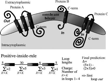
Topology of helical membrane proteins. Apolar helical segments are embedded in the lipid bilayer, perpendicular to its surface, as more or less rigid cylinders. Topology is "out" when the protein's N-terminus starts outside the cell (protein A) and "in" when it starts inside (proteins B and C). The lower part shows the positive-inside rule: if the even-numbered loops carry more positive charges, the N-terminus is predicted to be outside.
Why a window near 19? The oily core of a bilayer is about 30 Å thick, and an α-helix rises 1.5 Å per residue (unit 3), so crossing it takes about 20 residues. Here are three proteins with the transmembrane segments UniProt annotates from experiments: bacteriorhodopsin, a light-driven proton pump with seven; glycophorin A, a red-cell protein with one; and myoglobin, which stays in water.
import json, urllib.request
import numpy as np

KD = dict(I=4.5, V=4.2, L=3.8, F=2.8, C=2.5, M=1.9, A=1.8, G=-0.4, T=-0.7, S=-0.8, W=-0.9, Y=-1.3,
          P=-1.6, H=-3.2, E=-3.5, Q=-3.5, D=-3.5, N=-3.5, K=-3.9, R=-4.5)

def entry(accession):
    url = f"https://rest.uniprot.org/uniprotkb/{accession}.json"
    data = json.load(urllib.request.urlopen(url))
    spans = [(f["location"]["start"]["value"], f["location"]["end"]["value"])
             for f in data["features"] if f["type"] == "Transmembrane"]
    return data["sequence"]["value"], spans

def profile(seq, w=19):
    """Mean hydropathy of each window of w residues: a convolution with a box filter."""
    scores = np.array([KD[aa] for aa in seq])
    return np.convolve(scores, np.ones(w) / w, mode="valid")     # entry k covers residues k+1 .. k+w

def stretches(seq, w=19, threshold=1.6):
    """Residue ranges (1-based) covered by windows above the threshold, overlapping ranges merged."""
    runs = []
    for k in np.flatnonzero(profile(seq, w) > threshold):   # window k covers residues k+1 .. k+w
        first, last = int(k) + 1, int(k) + w
        if runs and first <= runs[-1][1] + 1:
            runs[-1] = (runs[-1][0], last)
        else:
            runs.append((first, last))
    return runs

proteins = {"bacteriorhodopsin": "P02945", "glycophorin A": "P02724", "myoglobin": "P02144"}
presets = []
for name, acc in proteins.items():
    seq, spans = entry(acc)
    print(f"{name} ({len(seq)} residues)")
    print("  annotated:", spans or "none")
    print("  predicted:", stretches(seq) or "none")
    presets.append({"name": name, "sequence": seq, "spans": spans})
bacteriorhodopsin (262 residues)
  annotated: [(23, 42), (57, 75), (93, 109), (121, 140), (148, 167), (186, 204), (217, 236)]
  predicted: [(24, 42), (57, 79), (119, 140), (148, 171), (218, 238)]
glycophorin A (150 residues)
  annotated: [(92, 114)]
  predicted: [(1, 23), (90, 115)]
myoglobin (154 residues)
  annotated: none
  predicted: none
A 19-residue window above 1.6 picks out five of bacteriorhodopsin's seven helices. The other two stay just under the line. The third helix, for example, carries two aspartates that relay protons across the membrane, and charged residues pull a window's average down. For glycophorin it finds the one membrane crossing and also a hydrophobic stretch at the very start that UniProt doesn't call transmembrane. That is a signal peptide, a hydrophobic tag that steers a new protein to the membrane and is then cut off, and hydropathy alone can't tell the two apart. Myoglobin gives nothing: its buried residues are spread along the sequence instead of collected in one 20-residue run.
Code
from primer import display_widget
display_widget("hydropathy", "Kyte–Doolittle profile; shaded bands are UniProt's transmembrane annotations.",
               presets=presets, window=19, threshold=1.6)
Kyte–Doolittle profile; shaded bands are UniProt's transmembrane annotations.
Amphipathic helices and the helical wheel
A helix in a soluble protein usually packs against the protein on one side and faces water on the other. Its sequence is amphipathic, hydrophobic on one face and polar on the opposite face, and a window average misses that because it averages both faces together. The signal is periodic. An α-helix turns once every 3.6 residues, so each residue sits 100° around the axis from the last, and residues i, i+3, i+4, and i+7 share a face. The helical wheel looks down the axis and places each residue at 100° from the previous one. The arrow is the hydrophobic moment, the sum of each residue's hydropathy as a vector pointing toward that residue: long when one face is oily, near zero when hydrophobic residues are scattered. It is the Fourier component of the hydropathy track at the helix's period.
Ubiquitin's one α-helix, Ile 23 to Glu 34. The crystal structure buries Ile 23, Val 26, Lys 27, and Ile 30,
positions i, i+3, i+4, and i+7, on the face the arrow points to (Lys 27's long carbon stem lies in
that face, with its charged tip in a salt bridge, lesson 2.4). Switch to 180° for the β-strand pattern, then
type ubiquitin's first strand, MQIFVKT, which buries Ile 3, Val 5, and Thr 7.
Helices that pack against each other in long bundles show the same idea with a slightly different period:
A coiled coil is a bundle of several helices assuming a side-chain packing geometry often referred to as "knobs-into-holes". The "knobs" are the side chains of one helix that pack into the hole created by four side chains surrounding the facing helix. This supercoil slightly alters the helix periodicity from 3.6 to 3.5 and results in the coiled-coil-specific symmetry in which every seventh residue occupies a similar position on the helix surface. The first and fourth of the seven residues are typically hydrophobic, the other four hydrophilic, frequently exposing the helix to solvent. These specific sequence features are at the base of accurate predictions for coiled coil helices.
Stretches that won't fold
Some stretches are built from very few letters: runs of glutamine, or long segments rich in S, G, E, and K. These low-complexity regions are often intrinsically disordered, never settling into one structure (lesson 3.5). The measure is a windowed Shannon entropy over the 20-letter alphabet, which collapses in a repetitive run. Two other quick reads: an even number of cysteines in a protein that works outside cells suggests disulfides, and clusters of G, P, N, D, and S mark turns and loops.
from collections import Counter
from primer import uniprot, fasta

def entropy(window):
    """Shannon entropy in bits of the residue distribution in a window (max log2(20) ≈ 4.32)."""
    counts = np.array(list(Counter(window).values()), dtype=float)
    p = counts / counts.sum()
    return float(-(p * np.log2(p)).sum())

header, htt = fasta(uniprot("P42858"))[0]       # human huntingtin
start = htt[:100]
print(start)
w = 12
h = [entropy(start[k:k + w]) for k in range(len(start) - w + 1)]
low = [k for k, e in enumerate(h) if e < 1.5]
print(f"windows below 1.5 bits start at residues {low[0] + 1}–{low[-1] + 1}")
print(f"entropy ranges from {abs(min(h)):.2f} to {max(h):.2f} bits")
MATLEKLMKAFESLKSFQQQQQQQQQQQQQQQQQQQQQPPPPPPPPPPPQLPQPPPQAQPLLPQPQPPPPPPPPPPGPAVAEEPLHRPKKELSATKKDRV
windows below 1.5 bits start at residues 15–70
entropy ranges from 0.00 to 3.08 bits
Huntingtin begins with a run of glutamines followed by a proline-rich stretch, and the entropy collapses over both. An expanded glutamine run is the cause of Huntington's disease.
From a string to label strings
The principal idea underlying most secondary structure prediction methods is the fact that segments of consecutive residues have preferences for certain secondary structure states. Thus, the prediction problem becomes a pattern classification problem tractable by pattern recognition algorithms. The goal is to predict whether a residue is in a helix, in a strand, or in none of the two (no regular secondary structure, often referred to as the "coil" or "loop" state).
The principal goal [of accessibility prediction] is to predict the extent to which a residue embedded in a protein structure is accessible to solvent. Different residues have a different possible accessible area. The most extreme simplification for accessibility accounts for this by normalizing (dividing observed value by maximally possible value) to a two-state description distinguishing between residues that are buried and exposed. The precise choice of the threshold is not well defined. The classical method to predict accessibility is to assign either of the two states, buried or exposed, according to residue hydrophobicity, that is, very hydrophobic stretches are predicted to be buried.
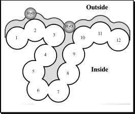
Residue solvent accessibility is measured by rolling a spherical water molecule over a protein surface and summing the area that can be accessed on each residue (typically 0 to 300 Ų). To compare long extended and compact amino acids, relative values are used (actual area as a percentage of the maximally accessible area). The simplified two-state description calls residues 1–3 and 10–12 here buried and 4–9 exposed.
Here are the true label strings for ubiquitin, from its crystal structure: secondary structure from the
HELIX and SHEET records of the PDB file, and burial (less than 20% relative accessibility, lesson 2.4).
from Bio.PDB.SASA import ShrakeRupley
from Bio.PDB.DSSP import residue_max_acc
from primer import structure, sequence, fetch

model = structure("1UBQ")[0]
chain = model["A"]
for res in [r for r in chain if r.id[0] != " "]:
    chain.detach_child(res.id)
ShrakeRupley().compute(model, level="R")
seq = sequence(chain)

ss = ["-"] * len(seq)                               # coil unless a record says otherwise
for line in open(fetch("1UBQ")):
    if line.startswith("HELIX"):
        first, last, label = int(line[21:25]), int(line[33:37]), "H"
    elif line.startswith("SHEET"):
        first, last, label = int(line[22:26]), int(line[33:37]), "E"
    else:
        continue
    for i in range(first, last + 1):
        ss[i - 1] = label

max_asa = residue_max_acc["Wilke"]
buried = ["b" if r.sasa / max_asa[r.get_resname()] < 0.2 else "-" for r in chain]
ruler = "".join(str(i // 10 % 10) if i % 10 == 0 else " " for i in range(1, len(seq) + 1))
print("       ", ruler)
print("seq    ", seq)
print("ss     ", "".join(ss))
print("buried ", "".join(buried))
                 1         2         3         4         5         6         7
seq     MQIFVKTLTGKTITLEVEPSDTIENVKAKIQDKEGIPPDQQRLIFAGKQLEDGRTLSDYNIQKESTLHLVLRLRGG
ss      EEEEEEE--EEEEEEEE-----HHHHHHHHHHHH-----EEEEEE--EEE-----HHHH----EEEEEEEEE----
buried  --b-b-b-----b-b-b---b-b--bb--b-----b----b-bbb----b----bb--b-b---b-b-b-------
Read down the columns. In the strands (E) burial alternates. In the helix (H, residues 23–34) the buried
positions are 23, 26, 27, and 30. The charged residues sit in the exposed columns. Three-state labels (H, E,
C) are the coarse version; unit 3 introduces the eight-state DSSP alphabet. A correct label string is still
not a structure: two proteins can share --EEEEE----EEEEE-- with their strands paired differently or in
different sheets.
Check yourself
A 300-residue protein's hydropathy plot (window 19) has two peaks above 1.6, one at residues 3–22 and one at 210–230. What are the possible readings, and what would you check?
Reasoning
The peak at 210–230 is a candidate transmembrane helix: about 20 residues, the right length to cross the bilayer. The N-terminal peak could also be a transmembrane helix, but a hydrophobic stretch right at the start is the classic signature of a signal peptide, which is cut off and doesn't stay in the membrane. Check for a signal-peptide cleavage site, or use a predictor that models signal peptides separately. Also check that the peaks hold up at window 19 and don't appear only at short windows.
An 18-residue peptide is very hydrophobic on average but has a hydrophobic moment near zero at 100°. A second peptide has a moderate average and a large moment. Which is more likely to lie along a membrane surface, half in and half out, and which to bury itself across the membrane?
Reasoning
The large-moment peptide has one oily face and one polar face, which suits lying flat at the interface between lipid and water, with the oily face down. Many antimicrobial peptides do exactly this. The uniformly hydrophobic peptide, with no face to keep in water, is the one that can sit inside the bilayer across the membrane, and at 18 residues it is close to long enough to span it.
Why does a window of 9 find surface loops of a soluble protein but a window of 19 doesn't, and why is the reverse true for transmembrane helices?
Reasoning
A window is a low-pass filter. Surface loops and buried stretches of soluble proteins alternate every 5 to 10 residues, so a 9-residue window resolves them, while a 19-residue window averages several of them together toward zero. A transmembrane helix is a single 20-residue block of hydrophobic residues. A 19-residue window matches its length and peaks clearly, while short windows also light up every small buried stretch of a soluble protein, which produces false alarms.